


![Helping Non-Security Stakeholders Understand ATT&CK in 10 Minutes or Less [VIDEO]](https://assets.crowdstrike.com/is/image/crowdstrikeinc/video-ATTCK2-1?wid=530&hei=349&fmt=png-alpha&qlt=95,0&resMode=sharp2&op_usm=3.0,0.3,2,0)
![Qatar’s Commercial Bank Chooses CrowdStrike Falcon®: A Partnership Based on Trust [VIDEO]](https://assets.crowdstrike.com/is/image/crowdstrikeinc/Edward-Gonam-Qatar-Blog2-1?wid=530&hei=349&fmt=png-alpha&qlt=95,0&resMode=sharp2&op_usm=3.0,0.3,2,0)


?wid=2048&hei=1350&fmt=png-alpha&qlt=95,0&resMode=sharp2&op_usm=3.0,0.3,2,0)


Motivation
Deep learning models have been considered “black boxes” in the past, due to the lack of interpretability they were presented with. However, in the last few years, there has been a great deal of work toward visualizing how decisions are made in neural networks. These efforts are saluted, as one of their goals is to strengthen people's confidence in the deep-learning-based solutions proposed for various use cases. Deep learning for malware detection is no exception here. The target is to obtain visual explanations of the decision-making — put another way, we are interested in the highlights that the model makes in the input as having potential malicious outcomes. Being able to explain these highlights from a threat analyst’s point of view gives a confirmation that we are on the right path with that model. We need to have the confidence that what we are building does not take completely random decisions (and get lucky most of the time), but rather that it has the right criteria for the required discrimination. With proof that the appropriate, distinctive features between malware and clean files are primarily considered during decision-making, we are going to be more inclined to give the model a chance at deployment and further improvements based on the results it has “in the wild.”
Context
With visualizations we want to confirm that a given neural network is activating around the proper features. If this is not the case, it means that it hasn’t learned properly the underlying patterns in the given dataset, and the model is not ready for deployment. A potential reaction, if the visualizations indicate errors in the selection of discriminative features, is to collect additional data and revisit the training procedure used. This blog focuses on convolutional neural networks (CNNs) — a powerful deep learning architecture with many applications in computer vision (CV), and in recent years also used successfully in various natural language processing (NLP) tasks. To be more specific, CNNs operating at the character level (CharCNNs) are the subject of visualizations considered throughout this article. You can read more about the motivation behind using CharCNNs in CrowdStrike’s fight against malware in this blog, “CharCNNs and PowerShell Scripts: Yet Another Fight Against Malware.” The use case is the same in the upcoming analysis: detecting malicious PowerShell scripts based on their contents, with a different target this time aimed at interpretability. The goal is to see through the eyes of our model and to validate the criteria on which its decisions are based.
One important property of convolutional layers is the retention of spatial information, which is lost in the upcoming fully connected layers. In CV, a number of works have asserted that deeper layers tend to capture more and more high-level visual information. This is why we use the last convolutional layer to obtain high-level semantics that are class-specific (i.e., malware is of interest in our case) with the spatial localization in the given input. Other verifications in our implementation are aimed at reducing the number of unclear explanations due to low model accuracy or text ambiguity. To address this, we take only the samples that are correctly classified, with a confidence level above a given decision threshold of 0.999.
Related Work
Among the groundbreaking discoveries leading to the current developments in CNN visualizations, there is proof (Zhou et al., 2015a) that the convolutional units in the CNNs for CV, act as object detectors without having any supervision on the objects’ location. This is also true in NLP use-cases, as the localization of meaningful words discriminative of a given class is possible in a similar way. Among the initial efforts towards CNN visualizations we can also mention the deconvolutional networks used by Zeiler and Fergus (2014) to visualize what patterns activate each unit. Mahendran and Vedaldi (2015) and Dosovitskiy and Brox (2015) show what information is being preserved in the deep features without highlighting the relative importance of this information. Zhou et al, 2015b propose CAM (class activation mappings) — a method based on global average pooling (GAP), which enables the highlighting of discriminative image regions used by the CNN to identify a given category. The direct applicability is in CV, as it is the case with most of the research done in this respect. However, it should be mentioned, once again, that the use cases extend to NLP as well, with a few modifications in the interpretations.
CAM has the disadvantage of not being applicable to architectures that have multiple fully connected layers before the output layer. Thus, in order to use this method for such networks, the dense layers need to be replaced with convolutional layers and the network re-trained. This is not the case with Grad-CAM (Selvaraju et al., 2016), Gradient-weighted CAM, where class-specific gradient information is used to localize important regions in the input. This is important as we want a visual explanation to be first, class-discriminative, meaning we want it to highlight the features (words/characters/n-grams) that are the most predictive of a class of interest which, in our case, would be malware.
Grad-CAM
Figure 1 offers a high-level view of how Grad-CAM is applied to textual inputs. Particularly, our interest is to visualize malicious PowerShell content in a heatmap fashion. In these visualizations, the most predictive features for malware are highlighted with different intensities according to their weights, from the perspective of our convolutional model. The following elements and actions are applicable in the mentioned Grad-CAM flow:
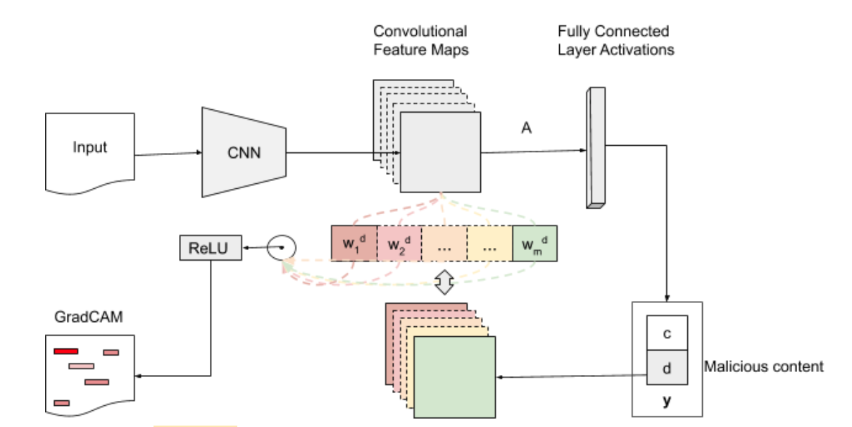 Figure 1: High-level view on the applicability of Grad-CAM for textual inputs. The more specific use-case hinted to in the diagram is heat map visualizations for malicious PowerShell scripts. (click image to enlarge)
- Inputs — in the current use-case the inputs provided are PowerShell scripts contents and the category of interest, which is malware in our case.
- Forward pass is necessary as we need to propagate the inputs through the model in order to obtain the raw class scores before softmax.
- Gradients are set to 0 for clean and 1 for malware (the class that is targeted).
- Backpropagate the signals obtained from the forward pass to the rectified convolutional feature map of interest, which is actually the coarse Grad-CAM localization.
- GradCAM outputs, in our case, are visualizations of the original scripts, with the most predictive features for the given class highlighted.
In Grad-CAM we try to reverse the learning process in order to be able to interpret the model. This is possible using a technique called gradient ascent. Instead of the regular weighted delta updates that are done to reduce the loss gradient x (-1) x lr, in gradient ascent, more delta is added to the area to be visualized in order to highlight the features of interest.
The importance of the k-th feature map for target class c is determined by performing Global Average Pooling (GAP) in the gradient of the k-th feature map: \< \alpha_k^c = \overbrace{\frac{1}{Z} \sum_{i}\sum_{j}}^{global\; average\; pooling} \underbrace{\frac{\delta y^{c}}{\delta A_{ij}^{k}}}_{gradients\; via\; backprop} \>
where
\( A_k \in \mathbb{R} ^ {u \times v} \) is the k-th feature map produced by the last convolutional layer, of width u and height v. \( y ^ c
\) — any differentiable activation (not only class scores), which is why Grad-CAM works no matter what convolutional architecture is used.
Global-average-pooling is applied on the gradients computed:
\< \frac{\delta y^{c}}{\delta A_{ij}^{k}} \>
Thus, we obtain the weights \( \alpha_k^c \), which represent a partial linearization of the deep network downstream from A and capture the importance of feature map k for a target class c.
Then we take the weighted average of the activation for each feature map. In order to do this, we multiply the importance of the k-th feature map:
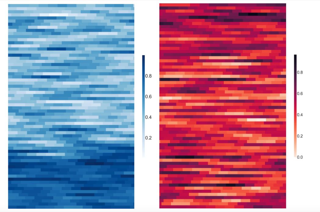 Figure 2: Heatmap visualizations of clean (left) and malicious (right) PowerShell files, resulted from GradCAM.
a. Inputs: the same as the inputs to the pre-trained CharCNN model b. Outputs:
i.The output to the final convolutional layer (previously determined) of the network ii. The output of the softmax activations from the model
3. In order to compute the gradient of the class output w.r.t. the feature map, we use GradientTape for automatic differentiation. 4. We pass the current sample through the gradient model and grab the predictions as well as the convolutional outputs. 5. Process the convolutional outputs such that they can be used in further computations (i.e., discard the batch dimension, evaluate the tensors, convert to numpy arrays if necessary, etc.). 6. Average the feature maps obtained and normalize between 0 and 1.Most Predictive Features
In order to justify the class-discrimination capabilities of our PowerShell model, we produce visualizations for both malware and clean samples, with a focus on the class of interest — malware. We consult with our threat analysts and conclude that many of the substrings highlighted in the samples are actually of interest in classifying maliciousness in scripts. Through this section, we are often going to refer to these highlights as substring matches. A strict selection is performed on all of the generated substring matches. These are checked against our Malquery database, with zero tolerance for false positives. Later, the substrings in the selected subset are considered for additional support to our PowerShell detection capabilities. The following sections briefly introduce three of the broadest categories of important substrings for our model in deciding the maliciousness of PowerShell scripts.Base64 Strings
Substring 1:piJ0DAIB9EAB0seuZZotF3GaJh4gAAADrtmaLReBmiYeKAAAA665Vi+yhtGdMAItNGIP4AQ+FwZ4DAItFCIP4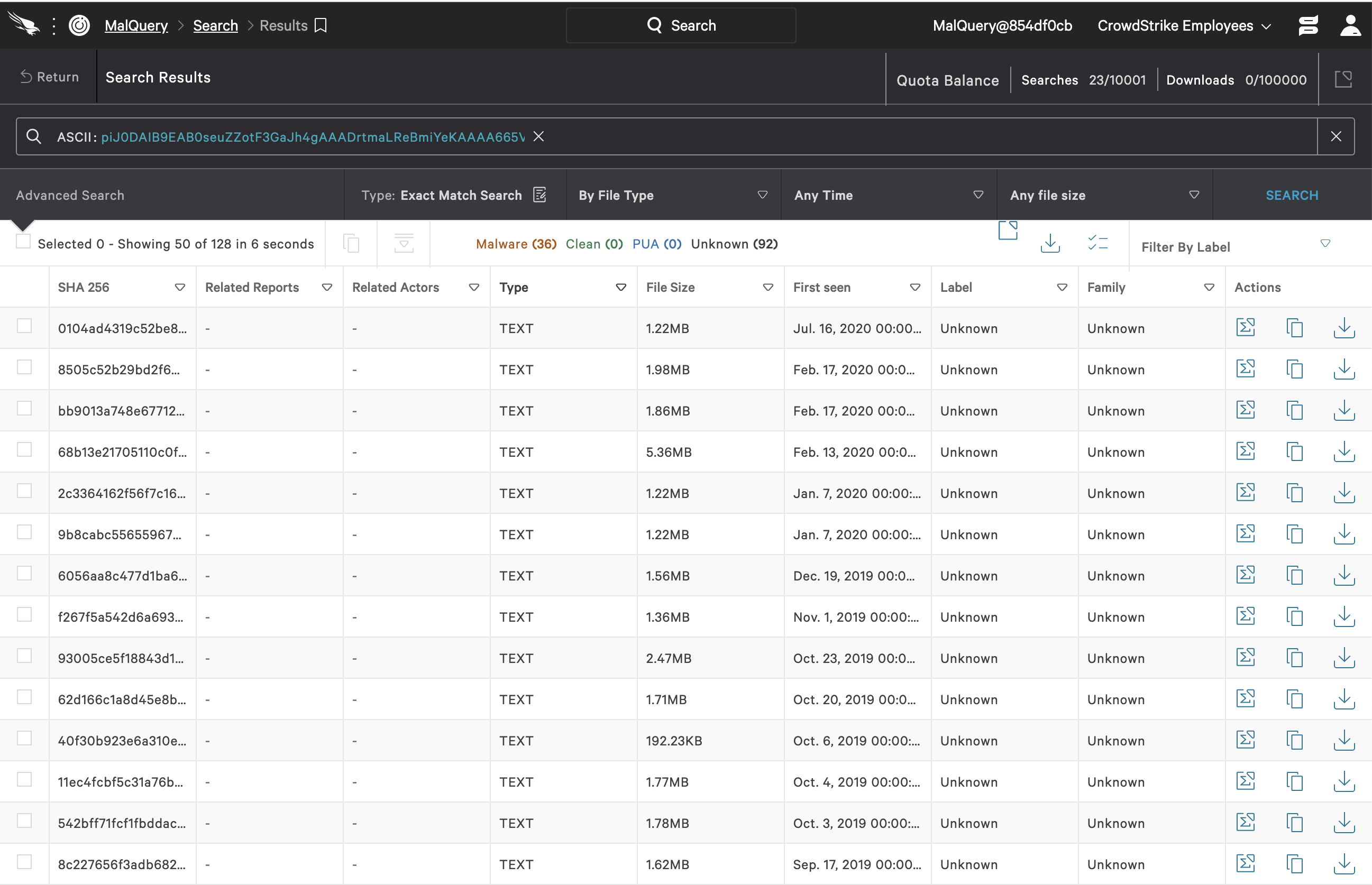 Click image to enlarge.
Common Syntax
Substring 2:IEX (New-Object IO.StreamReader(New-Object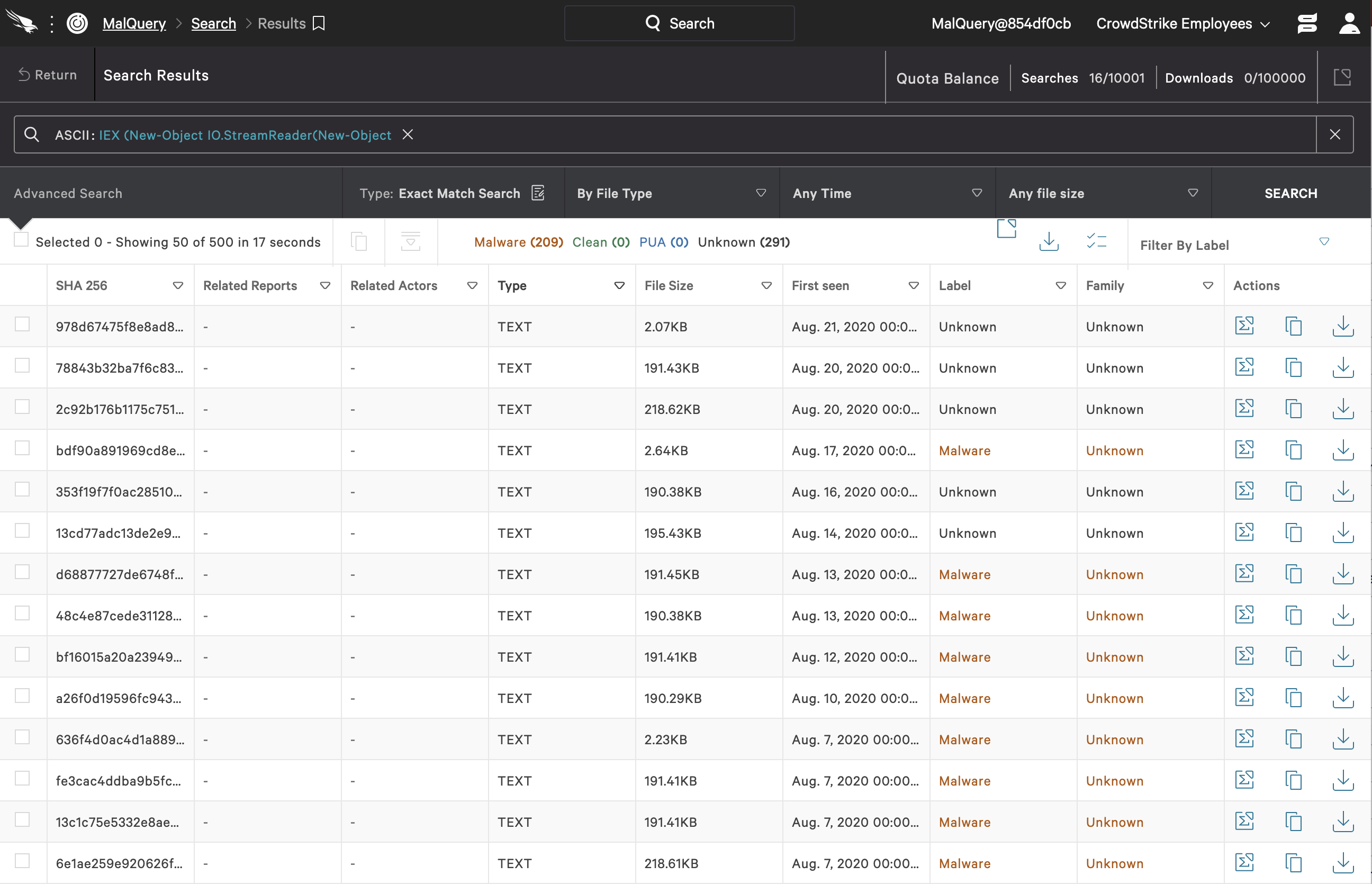 Click image to enlarge.
IO.Compression.CompressionMode>::Decompress))).ReadToEnd()))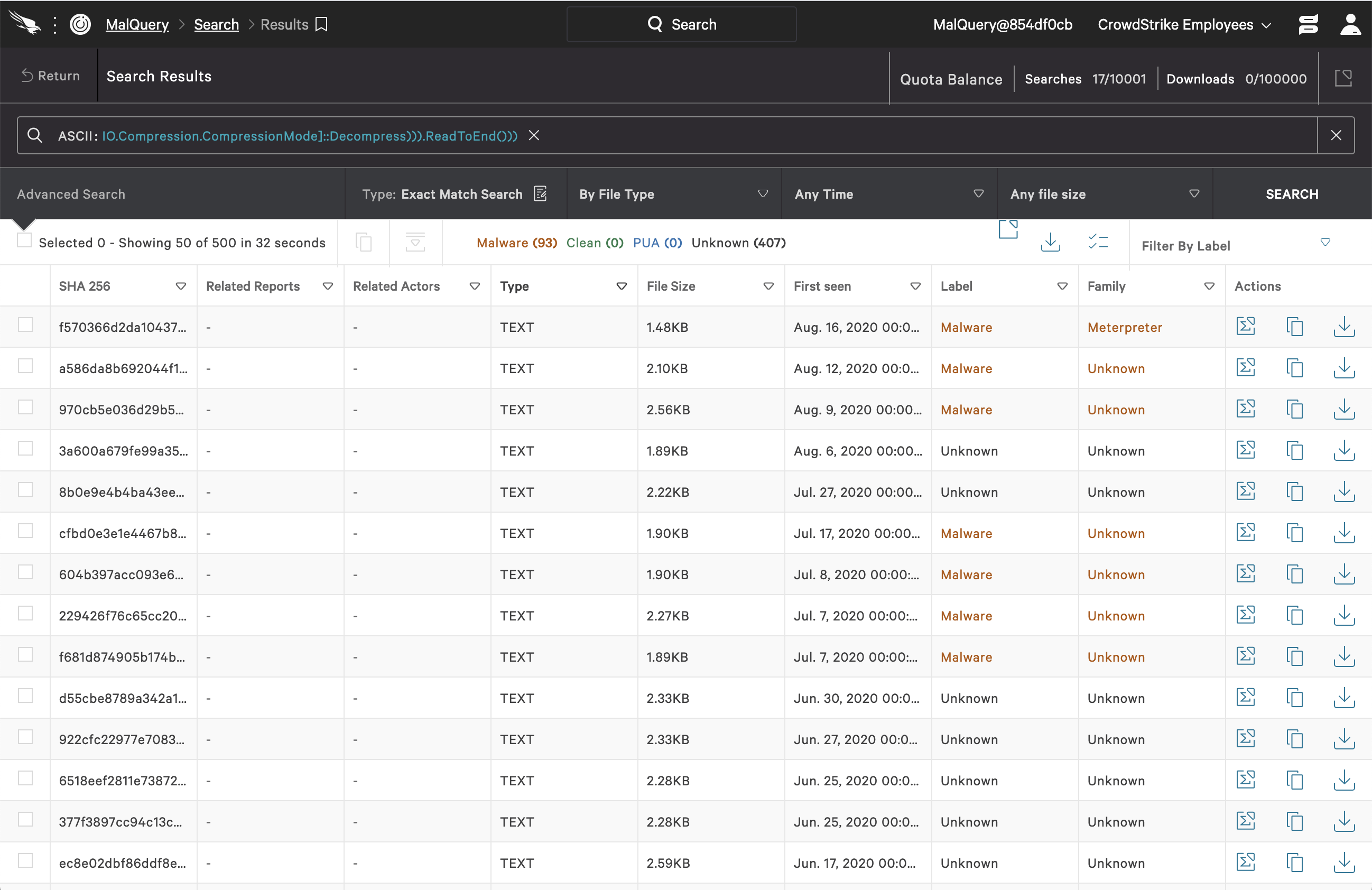 Click image to enlarge.
powershell /w 1 /C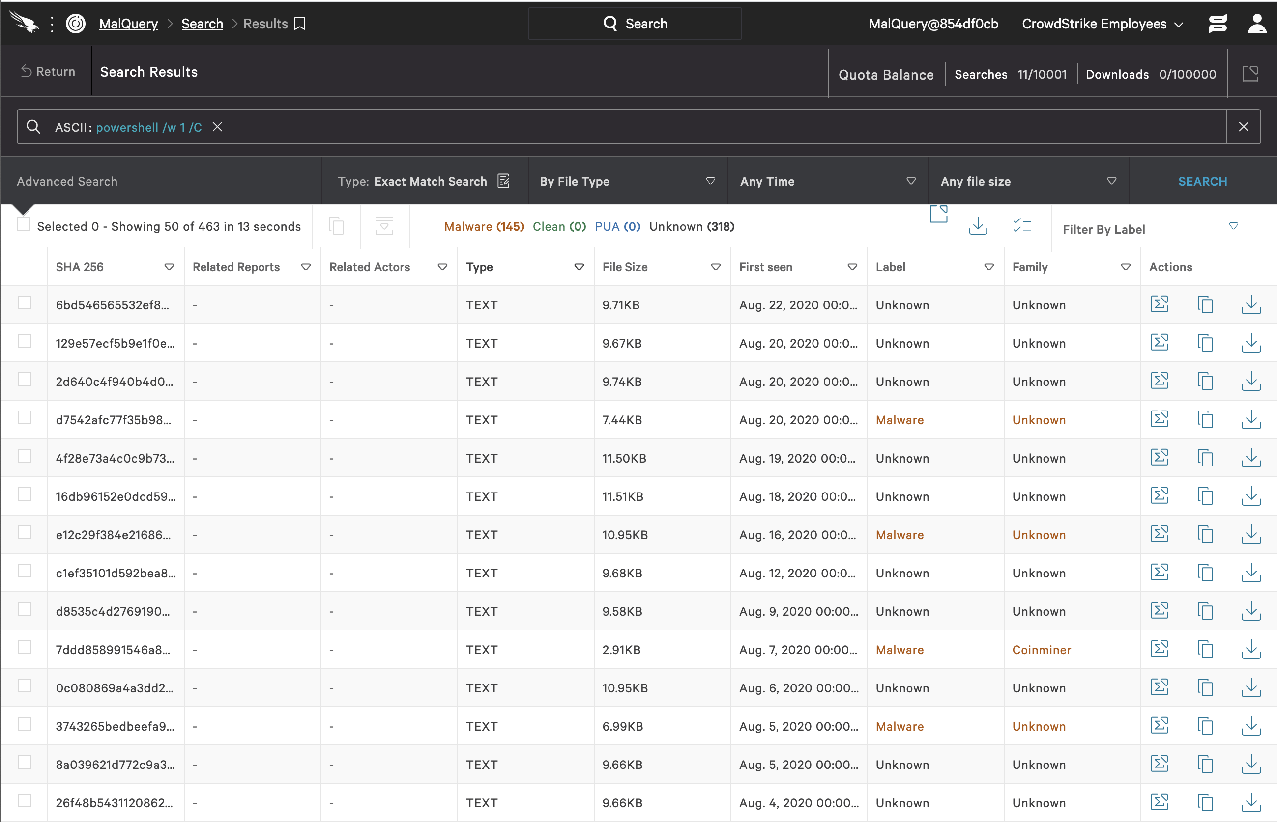 Click image to enlarge.
Common Obfuscation
Obfuscation techniques for Windows Portable Executables are also detected as significant strings in our model. It is clear why attackers would try to obfuscate other executions launching from within the current script. Two such examples selected from our set of potential templates are Substring 5 and Substring 6. Substring 5:Chr(Asc("x")) + Chr(Asc(“e”))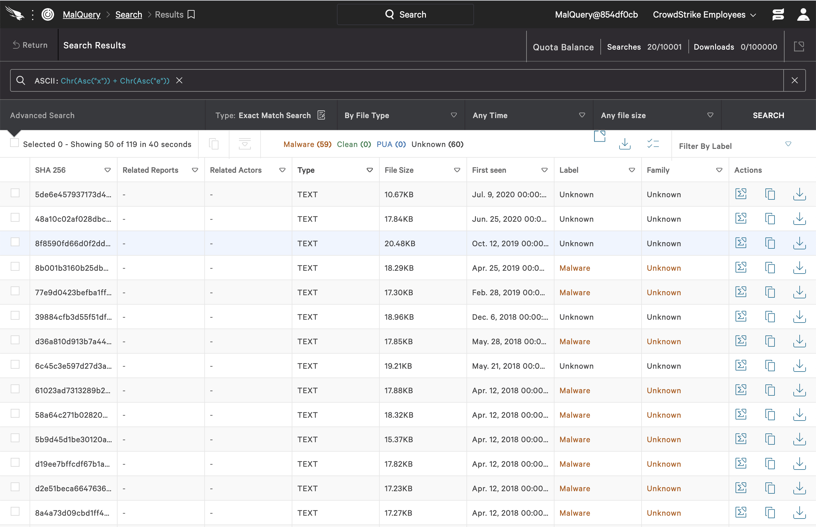 Click image to enlarge.
Chr(101) & "xe';"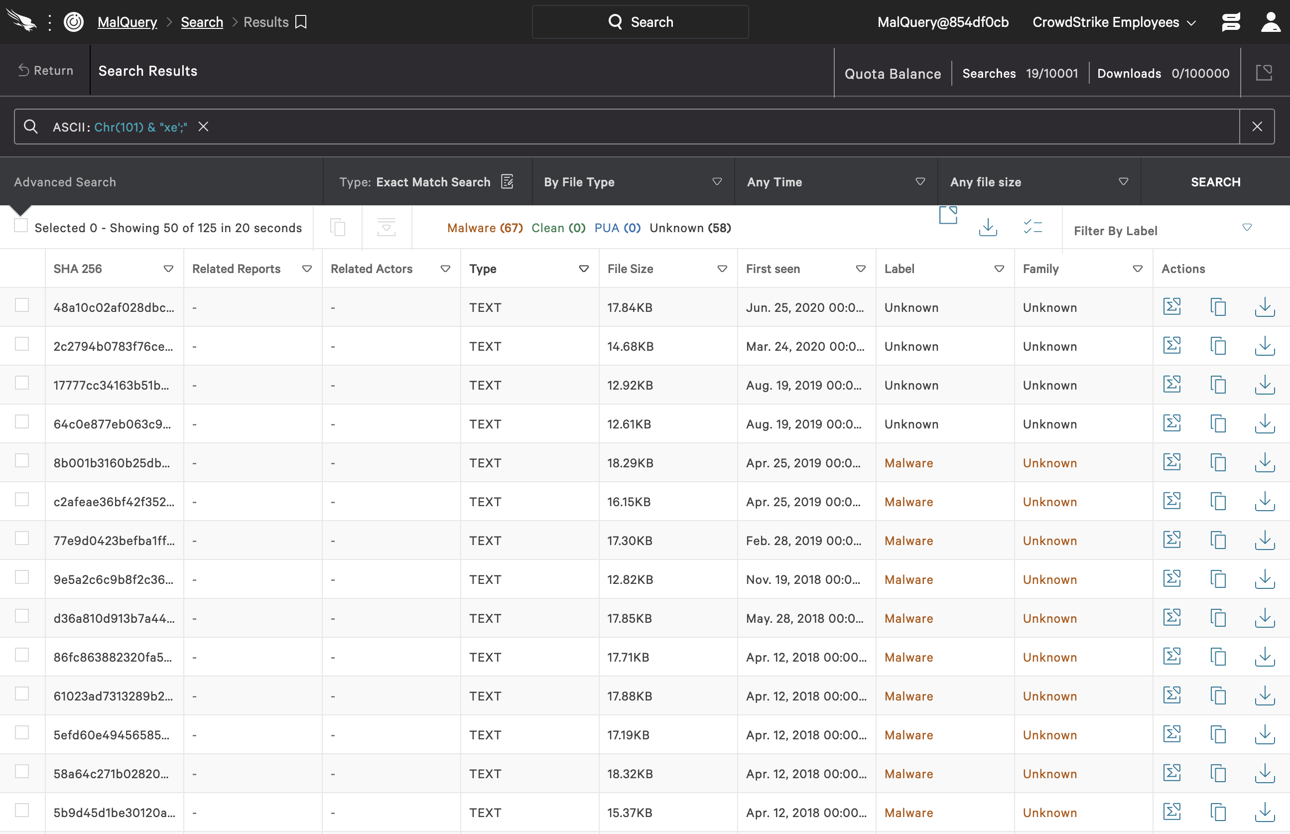 Click image to enlarge.
Conclusion
In this blog we introduced a visualization technique that exploits the explainability potential of convolutional neural networks. The context, motivation and importance of seeking interpretability in our models were also discussed. We briefly described the components and flow in a visualization technique coming from the computer vision domain, namely Grad-CAM. By employing this technique with additional filtering, we can obtain a set of malware predictive substrings that further complement our current detection capabilities for PowerShell scripts. A few examples of such substrings are discussed at length in this article.Additional Resources
- Read about the CrowdStrike Falcon® Malquery malware search engine.
- Learn more about the CrowdStrike Falcon® platform by visiting the product page.
- Test CrowdStrike next-gen AV for yourself. Start your free trial of Falcon Prevent™ today.


