


![Helping Non-Security Stakeholders Understand ATT&CK in 10 Minutes or Less [VIDEO]](https://assets.crowdstrike.com/is/image/crowdstrikeinc/video-ATTCK2-1?wid=530&hei=349&fmt=png-alpha&qlt=95,0&resMode=sharp2&op_usm=3.0,0.3,2,0)
![Qatar’s Commercial Bank Chooses CrowdStrike Falcon®: A Partnership Based on Trust [VIDEO]](https://assets.crowdstrike.com/is/image/crowdstrikeinc/Edward-Gonam-Qatar-Blog2-1?wid=530&hei=349&fmt=png-alpha&qlt=95,0&resMode=sharp2&op_usm=3.0,0.3,2,0)


?wid=2048&hei=1350&fmt=png-alpha&qlt=95,0&resMode=sharp2&op_usm=3.0,0.3,2,0)


In this blog, we present the results of some preliminary experiments with training highly “overfit” (interpolated) models to identify malicious activity based on behavioral data. These experiments were inspired by an expanding literature that questions the traditional approach to machine learning, which has sought to avoid overfitting in order to encourage model generalization.
The results discussed here, although preliminary, validate that the insights of this new literature seem to apply to our problem domain, and that perhaps training highly overfit models on our behavioral data will yield the best possible performance.
The Traditional Approach to Generalization
At CrowdStrike, we are constantly training, experimenting on and deploying new machine learning models as part of our efforts to identify and prevent malicious activity. A critical concern in these efforts is training models that generalize well — that is, models that perform well not just on the data the model is trained over but also on data not included in the training set. In the cybersecurity setting, generalization is what allows a model to detect never-before-seen malware and learn latent characteristics identifying malicious activities. Encouraging generalization is often thought of in terms of its (almost) converse: overfitting. A model is thought of as overfit when it learns spurious rules that leverage the data's high dimensionality to perfectly fit its training labels (note this definition is inherently imprecise, as whether a learned rule is overfit or "true" is in many ways based on interpretation). The more complexity and degrees of freedom a model has, the more ability it has to overfit the data.
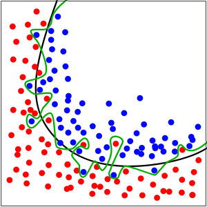 Figure 1: Overfit model (green line) vs generalizable model (black line) in a binary classification problem (Image source: https://en.wikipedia.org/wiki/Overfitting)
Figure 1 is a classic example of overfitting. The green and black lines each represent a model trained to classify the red and blue data points. The green line, while perfectly fitting the data, is thought to be overfit, while the smoother black line presumably has better generalization performance.
Traditionally, statistics and machine learning think of improving generalization (given a fixed data set) and avoiding overfitting as one and the same. Techniques to avoid overfitting are broadly known as regularization, because often they operate by enforcing simpler models or penalizing complexity in the course of training. The relationship between overfitting and generalization is often thought of in terms of the bias/variance trade-off:
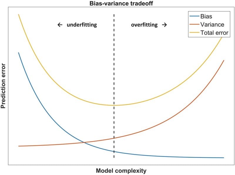 Figure 2. The classic bias-variance trade-off: As model complexity increases, performance on the training data continues to improve, but is eventually overshadowed by degradation in generalization performance. (Source: Dankers, Traverso, Wee et al. <1>)
Avoiding Overfitting May Not Always Help
The quickly expanding literature has raised many questions about the universality of the bias-variance trade-off and the traditional understanding that preventing overfitting is a requirement of out-of-sample performance. While this literature was originally born in the deep learning for image classification space, it has been shown to apply to an ever-wider range of problems. While we won't attempt a review of the literature here, we will summarize some key points:
- Across many problem domains, models that heavily overfit the training data perform better than the best models that do not. This observation has been replicated across many problem domains and model architectures, including the kinds of boosted tree models experimented with here. (<2>,<3>,<4>,<5>,<6>
- )Performance on held-out data (aka generalization performance) seems to exhibit a double dip, wherein the generalization performance degrades as a model and becomes overfit (the usual bias-variance trade-off), but improves again as the model continues to overfit the training data (the interpolating regime).
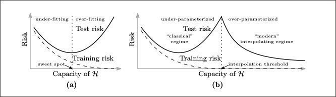 Figure 3. Curves for training risk (dashed line) and test risk (solid line). (a) The classical U-shaped risk curve arising from the bias-variance trade-off. (b) The double descent risk curve, which incorporates the U-shaped risk curve (i.e, the “classical” regime) together with the observed behavior from using high-capacity function classes (i.e., the “modern” interpolating regime), separated by the interpolation threshold. The predictors to the right of the interpolation threshold have zero training risk. (Source: Belkin, Hsu, Ma, and Mandal <3>)
 - The extent of these effects is driven in a complex and not well-understood way by the underlying complexity of the data, capacity of the model and relative size of the training data set. This has resulted in seemingly counterintuitive results such as better models being trained from smaller data sets.
- The gains from training overfit models may require that the true data distribution is long-tailed and the trained models are sufficiently complex. (<6>)
Interpolation and Our Data
Of course, our first thought is, how does this new literature apply to our problem? Cybersecurity data exhibits many of the characteristics that may be important in determining the effectiveness of regularization vs. overfit models:
- Cybersecurity data is extremely "long-tailed": The distribution of behaviors and files and other data has immense variety, and it is common to see relatively uncommon/unique data points.
- For many cybersecurity problems, it is hard to know if even extremely large data sets are truly large relative to the inherent data complexity.
- Many of our models have the capacity to perfectly fit training data.
However, because this literature is so new and still quite active, it is far from clear if our model generalization can benefit from training to highly overfit. Our goal with the experiments discussed next is to begin to answer this question.
The Problem Space
We focus here on the specific task of training a boosted tree model on process-level behavioral data to identify malicious activity. This behavioral data consists of a huge variety of events attempting to capture everything that a process did on a system. These descriptions of behaviors can be aggregated together for a single process and turned into numeric features. The result is a feature vector where each numeric value represents a separate feature. As an example, a feature vector like
(5.7, 1, 0, 3, 4, 1, ..., 56.789, ...) might mean that the process ran for 5.7 seconds of kernel time, created a user account, did not write any files, made three DNS requests, etc. In our specific case, our feature vector has on the order of 55,000 features. As a result, even though the space of possible behaviors is vast, a priori it appears likely that our model is sufficiently complex to perfectly fit our training data.
- Behavioral data is long-tailed.
- Our training data set is necessarily small, relative to the extremely long tail of possible behavior.
- We train complex models with relatively high dimensions of features.
Our Experiments
We experiment with training memorized/overfit versions of a boosted tree model trained over the behavioral data described above. In our typical training regime, we actively attempt to avoid overfitting. In the case of the models here, that is primarily accomplished by including regularization terms in the loss functions, restricting the depths of trees, and early stopping (carefully monitoring model performance on held-out data, and ending training once the model is no longer improving performance on the holdout set). For this experiment:
- We remove all regularizing parameters.
- Increase the maximum depth of trees trained at each round.
- And most importantly, continue training for many iterations without regard to the models’ performance on the test set.
We also compare the model performance to a "traditionally" trained model with regularization and early stopping.
So, how do our interpolated models perform?
The Surprising (or Not?) Performance of Our Interpolated Models
It turns out even with these limited initial experiments, we generate some compelling results and are able to observe many of the characteristic features noted in the interpolation literature. In particular, we observe:
- The "double dip" phenomenon in model performance.
- Model performance continues to improve well after the model has fully memorized the training data.
Results
The first thing to note is that after 500 rounds of boosting with no regularization and deep trees, we do indeed appear to have a model that is solidly in the interpolation regime. This can be seen in the model's performance on the training set as we add trees (e.g., iterate through boosting rounds). In fact, the model is able to perfectly classify the training data well before the hundredth round of boosting. Unfortunately, the observed log loss on the held-out data does not obviously exhibit the "double dip" described in the literature. Rather, the log loss on the holdout (test) data seems to imply that the classical approach is true: The best performance in terms of log loss appears to be reached early on and then degrade as the model continues to fit the training data, as seen in Figure 4.
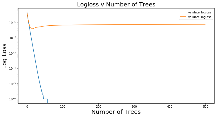 Figure 4. Log loss on training data vs holdout (test) data as trees are added and model complexity is increased
But wait! Although we use log loss as the objective to minimize in training, we do not really care about it in practice. Instead, we care how well our model can identify malicious activity (true positive rate) without generating too many false positives. In other words, better models achieve higher true positive rates (TPRs) at any given false positive rate (FPR). When we apply this reasoning and visualize how the model's TPR for a fixed FPR evolves as we add trees to the model, we immediately see the characteristic double dip: The TPR increases, reaches a peak, and then falls, consistent with the traditional bias-variance trade-off story. However, after the model has already reached perfect classification on the training data (0 log loss), the TPR on the holdout data continues to rise. This rise continues for hundreds of additional boosting rounds, even though the model has seemingly trained to completion on the training data. It should be stressed how surprising this is from the perspective of traditional bias-variance trade-off, and it validates that the literature on the performance of interpolated models applies to our domain.
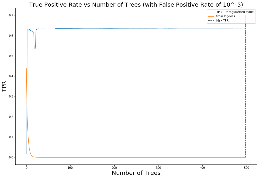 Figure 5. Evolution of TPR at a fixed FPR of 0.0001 as trees are added to the model to increase complexity
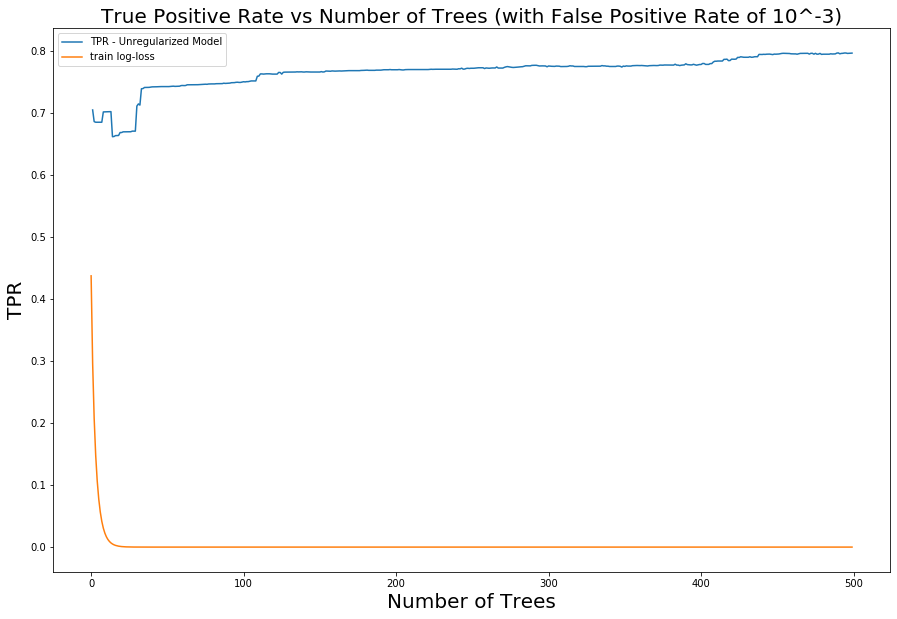 Figure 6. Evolution of TPR at a fixed FPR of 0.001 as trees are added to the model to increase complexity
More generally, we can observe the evolution of model performance across the entire range of FPRs by visualizing how the model's receiver operating characteristic (ROC) curves (graphs of TPR vs. FPR) shift as we iterate over the number of trees.
 Figure 7. Evolution of ROC curves as trees are added to the model
Comparison to Other Models
Unfortunately, our interpolated model does not perform as well as our benchmark model trained using regularization and early stopping. However, this is likely simply a reflection of the limited nature of our experimentation, rather than a repudiation of the performance of an interpolated model. Specifically:
- Our benchmark model was trained with near-optimal hyper-parameters resulting from extensive hyper-parameter search, whereas we have done no hyper-parameter tuning on the interpolated model.
- Our interpolated model was still improving in the latest rounds of training. It is likely that with additional trees, it would yield an even higher performance.
As a result, given our observations here it appears likely that with some additional experimentation, an interpolated model can be trained that outperforms our benchmark.
Conclusions and Next Steps
What can we take away from this small bit of experimentation? And what are the limitations of what we have done here?
- We know: Interpolation really does result in improved performance beyond the traditional bias-variance performance peak in our domain. Models definitely improve well into the interpolating regime.
- We do not know: if interpolated models are the best because we have not exhaustively searched through possible hyper-parametrizations or benchmarked against all possible regularized models.
While these results are very preliminary, they are compelling enough to warrant further investigation. In particular, it appears plausible that an appropriately tuned interpolated model may achieve the peak generalization performance out of all possible models.
Citations and Sources
- Dankers FJWM, Traverso A, Wee L, et al. Prediction Modeling Methodology. 2018 Dec 22. In: Kubben P, Dumontier M, Dekker A, editors. Fundamentals of Clinical Data Science . Cham (CH): Springer; 2019. Fig. 8.3, . Available from: https://www.ncbi.nlm.nih.gov/books/NBK543534/figure/ch8.Fig3/ doi: 10.1007/978-3-319-99713-1_8
- Mikhail Belkin, Alexander Rakhlin, Alexandre B. Tsybakov. Does Data Interpolation Contradict Statistical Optimality? https://arxiv.org/abs/1806.09471
- Mikhail Belkin , Daniel Hsu , Siyuan Ma , and Soumik Mandal. Reconciling modern machine learning practice and bias-variance trade-off. https://arxiv.org/pdf/1812.11118.pdf
- Trevor Hastie, Andrea Montanari, Saharon Rosset, Ryan J. Tibshirani. Surprises in High-Dimensional Ridgeless Least Squares Interpolation. https://arxiv.org/pdf/1903.08560.pdf
- Adam J Wyner, Matthew Olson, Justin Bleich. Explaining the Success of AdaBoost and Random Forests as Interpolating Classifiers. https://arxiv.org/pdf/1504.07676.pdf
- Vitaly Feldman. Does Learning Require Memorization? A Short Tale about a Long Tail. https://arxiv.org/pdf/1906.05271.pdf
Additional Resources
- If you’re ready to work on unrivaled technology that’s processing data at unprecedented scale, please check out our open engineering and technology positions.
- Learn more about the CrowdStrike Falcon® platform by visiting the product page.
- Test CrowdStrike next-gen AV for yourself. Start your free trial of Falcon Prevent™ today.


