


![Helping Non-Security Stakeholders Understand ATT&CK in 10 Minutes or Less [VIDEO]](https://assets.crowdstrike.com/is/image/crowdstrikeinc/video-ATTCK2-1?wid=530&hei=349&fmt=png-alpha&qlt=95,0&resMode=sharp2&op_usm=3.0,0.3,2,0)
![Qatar’s Commercial Bank Chooses CrowdStrike Falcon®: A Partnership Based on Trust [VIDEO]](https://assets.crowdstrike.com/is/image/crowdstrikeinc/Edward-Gonam-Qatar-Blog2-1?wid=530&hei=349&fmt=png-alpha&qlt=95,0&resMode=sharp2&op_usm=3.0,0.3,2,0)


?wid=2048&hei=1350&fmt=png-alpha&qlt=95,0&resMode=sharp2&op_usm=3.0,0.3,2,0)


Machine learning for computer security has enjoyed a number of recent successes, but these tools aren’t perfect, and sometimes a novel family is able to evade file-based detection. This blog walks you through a method to automatically extract discriminative features from the entry point of portable executable (PE) malware — in this case, malware binaries in the “Portable Executable” format used by Microsoft Windows. We show that these features can be used to augment an existing feature space to boost the effectiveness of a model, especially for troublesome malware families. We call this method a “MALE Model” — Machines Automatically Learning Embedding Models — for reasons that may be best explained by the film Zoolander (2001) with these quotes.
Sometimes, machine learning models will make a mistake. In the case of a novel malware family, the model might be deceived if samples from this novel family are closer to the benign software than the malicious software in the training set. Sometimes, models are easily deceived. For example, William Fleshman recently had success creating evasive malware by appending well-chosen strings to malware files. Fleshman’s attack works because the machine learning model assumes that files containing those well-chosen strings (such as a Microsoft end-user license agreement, or EULA) must be clean. Of course, this assumption is blatantly false, but machine learning is an imperfect endeavor. I've examined this phenomenon in the past, and wrote about one proposed solution to additive evasions of this type.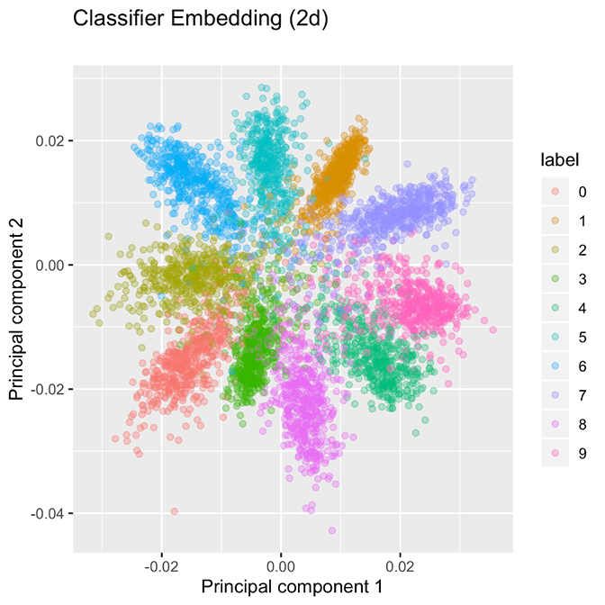 Figure 1. Classification networks separate classes, but the groupings are tightly packed.
By contrast, the embedding strategy produces well-separated family clusters, as shown in Figure 2. The contrast suggests two alternative approaches to creating groupings. The classification model shown in Figure 1 appears to be segmenting ℝ² into 10 “wedges,” one for each class, while the embedding network shown in Figure 2 will create a tight bubble for each class. As opposed to wedges, these bubbles are not exhaustive on ℝ², so we anticipate that the arrival of a new class, such as hexadecimal digits A, B, C, …, F will be allocated to their own bubbles because CNNs are able to extract useful low-level concepts about handwritten characters and use that information to distinguish among digits. These facts are a direct consequence of the loss function used for embeddings.
Figure 1. Classification networks separate classes, but the groupings are tightly packed.
By contrast, the embedding strategy produces well-separated family clusters, as shown in Figure 2. The contrast suggests two alternative approaches to creating groupings. The classification model shown in Figure 1 appears to be segmenting ℝ² into 10 “wedges,” one for each class, while the embedding network shown in Figure 2 will create a tight bubble for each class. As opposed to wedges, these bubbles are not exhaustive on ℝ², so we anticipate that the arrival of a new class, such as hexadecimal digits A, B, C, …, F will be allocated to their own bubbles because CNNs are able to extract useful low-level concepts about handwritten characters and use that information to distinguish among digits. These facts are a direct consequence of the loss function used for embeddings.
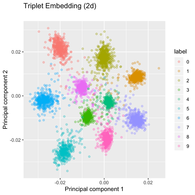 Figure 2. In an embedding network, classes are allocated to well-separated groupings. The embedding network uses a margin of 0.2 in the original space.
These figures were created using nearly the same network. The only differences are (1) the loss function used, and (2) the classification network has one additional layer after the two-dimensional embedding to give predicted probabilities. Presently, we discuss how the embedding network’s loss function must yield well-separated clusters. Indeed, if we compute the batch-hard triplet loss of the classification network depicted in Figure 1, it achieves a loss of 16.33 on the validation data, whereas the embedding network, which is explicitly minimizing the batch-hard triplet loss, achieves a dramatically lower loss of 0.1261 (the embedding network uses a margin α = 0.2). The reason for this wide discrepancy is that the triplet loss function encourages well-separated groupings which are more suited to minimizing the triplet loss.
Creating an embedding from family labels requires a specialized loss function. Following the suggestions in the FaceNet paper, we can state our goal mathematically as
Figure 2. In an embedding network, classes are allocated to well-separated groupings. The embedding network uses a margin of 0.2 in the original space.
These figures were created using nearly the same network. The only differences are (1) the loss function used, and (2) the classification network has one additional layer after the two-dimensional embedding to give predicted probabilities. Presently, we discuss how the embedding network’s loss function must yield well-separated clusters. Indeed, if we compute the batch-hard triplet loss of the classification network depicted in Figure 1, it achieves a loss of 16.33 on the validation data, whereas the embedding network, which is explicitly minimizing the batch-hard triplet loss, achieves a dramatically lower loss of 0.1261 (the embedding network uses a margin α = 0.2). The reason for this wide discrepancy is that the triplet loss function encourages well-separated groupings which are more suited to minimizing the triplet loss.
Creating an embedding from family labels requires a specialized loss function. Following the suggestions in the FaceNet paper, we can state our goal mathematically as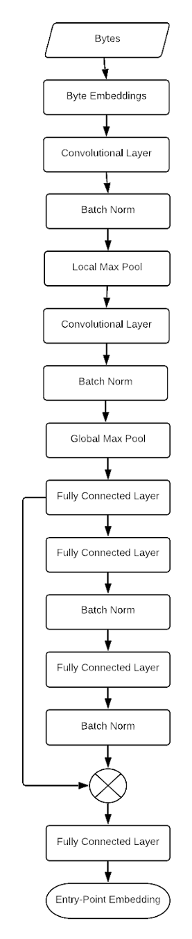 Figure 3. Diagram of CNN architecture to create embeddings of software directly from the raw bytes of the file.
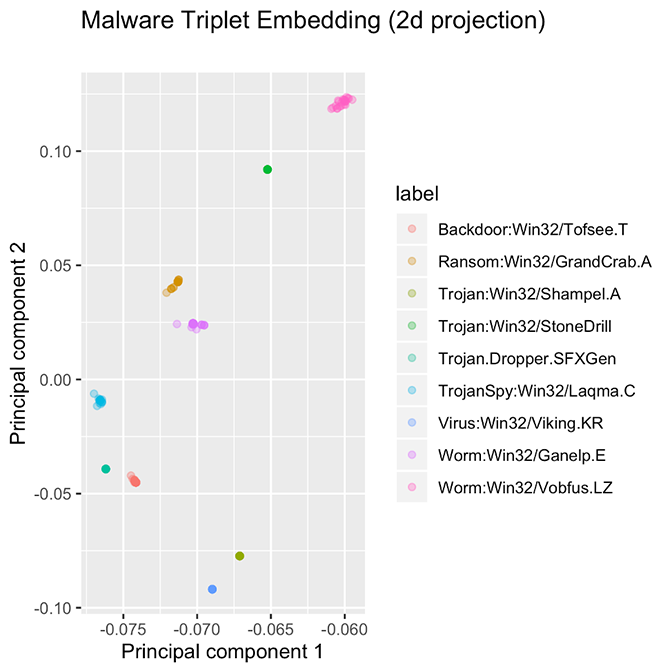 Figure 4. Ten families, each with approximately 25 samples. Some families are so tightly packed that all examples overlap at the same point. The ten families presented here are good examples of what we would like to achieve with PE file embeddings.
These methods aren’t perfect, however. We observe two failure modes, presented in Figure 5. In one class of failures, some families did not cluster at all, no matter which model or hyperparameter configuration we used. We hypothesize that the samples in this family have very different entry points, or that the supposed “family” is very noisy and does not conform to the idea of similarity that we expect from a family of software samples.
Figure 4. Ten families, each with approximately 25 samples. Some families are so tightly packed that all examples overlap at the same point. The ten families presented here are good examples of what we would like to achieve with PE file embeddings.
These methods aren’t perfect, however. We observe two failure modes, presented in Figure 5. In one class of failures, some families did not cluster at all, no matter which model or hyperparameter configuration we used. We hypothesize that the samples in this family have very different entry points, or that the supposed “family” is very noisy and does not conform to the idea of similarity that we expect from a family of software samples.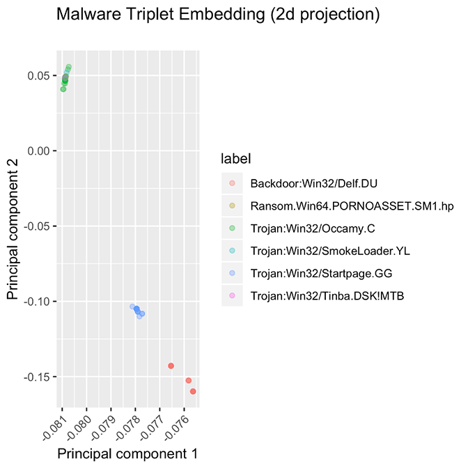 Figure 5. These families are some examples of “failure modes” for the embedding model. Some families are spread out over a wide range of values, instead of being tightly packed, while other families are stacked atop each other.
For both failure modes, it will be fruitful to investigate these hypotheses, since determining the cause of these “misfits” could lead to an improved taxonomy of malware. For example, it would be interesting to know if the same custom packer were used for several different malware families. (We verify that these visual results aren’t a trick of the choice of projection by computing distances between samples and finding that samples from distinct families are very close, relative to the margin parameter in the original embedding space.)
Figure 5. These families are some examples of “failure modes” for the embedding model. Some families are spread out over a wide range of values, instead of being tightly packed, while other families are stacked atop each other.
For both failure modes, it will be fruitful to investigate these hypotheses, since determining the cause of these “misfits” could lead to an improved taxonomy of malware. For example, it would be interesting to know if the same custom packer were used for several different malware families. (We verify that these visual results aren’t a trick of the choice of projection by computing distances between samples and finding that samples from distinct families are very close, relative to the margin parameter in the original embedding space.)
Table 1. Experimental results show that using embeddings to augment the classifier provides a statistically significant improvement to the model. The best model for each task is bolded. Brackets show 95% confidence intervals.
Likewise, we are impressed that the embedding features improve the classification of this novel family in comparison to a model trained without these features. We suspect that this is because the embeddings are constructed by accounting for the presence or absence of different distinguishing features of the entry-point data, so in a limited, highly abstract way, the network can interpret the familial hallmarks of the software.
We’ve introduced and analyzed a convolutional embedding network to augment machine learning classifiers and improve classification of novel malware families. We believe that this general method of creating embedding representation of PE files can be extended to many other areas, such as similarity search, novelty detection, cross-platform transfer learning, and discovery of new families.
David J. Elkind is a senior data scientist at CrowdStrike and holds an M.S. in mathematics from Georgetown University.
But what can we do to make malware models robust in a more general setting, where we don’t necessarily know or have the ability to simulate whatever traits make the novel malware family evasive? Or, if we have a classifier that does well overall, but poorly on a specific malware family, how can security researchers discover new features to correctly distinguish between benign software and malware? In this blog post, I propose a very general feature extraction method that can be used to augment existing features to address both of those shortcomings.
Convolutional Neural Networks for Software Consume Raw Bytes
The standard approach to classifying new malware is also the simplest: Just retrain the model with the new samples. Model retraining is helpful when you have enough new malware samples to work with to establish a clear signal, but there are shortcomings with this approach. If the feature space isn’t rich enough to distinguish some malware families from clean software, model retraining won’t be able to fix it because of the overlap between the two classes in the feature space. On the other hand, adding new features can increase the discriminative power of the network. One way to approach this problem is to have someone skilled in malware analysis undertake feature engineering, the process of gathering raw information for use by machine learning to distinguish benign software from malware. Feature engineering is a hard problem that involves reverse engineering the samples and putting together some features that identify whatever those samples have in common, and what distinguishes those samples from other software. For an example of how we do this at CrowdStrike, see the blog Gimme Shellter, which explains how Shellter is used to bypass antivirus products. The expense and complexity of human-engineered features make this task an attractive candidate for automation. We show that modern machine learning methods can be leveraged to fill this niche. Computer security researchers have successfully used convolutional neural networks (CNNs) to classify raw binaries directly, without relying on humans to handcraft feature vectors. Some examples include:- "Malware Detection by Eating a Whole EXE," Edward Raff, Jon Barker, Jared Sylvester, Robert Brandon, Bryan Catanzaro and Charles Nicholas
- “Deep Convolutional Malware Classifiers Can Learn from Raw Executables and Labels Only,” Marek Krčál, Ondřej Švec, Martin Bálek and Otakar Jašek
- "What are Deep Neural Networks Learning About Malware?" Scott Coull and Christopher Gardner
Embedding Networks Produce Widely Separated Groupings
We reason that family embeddings will improve the downstream classification task because a successful family embedding will, by construction, isolate families. With novel families isolated, the classifier can use that information to differentiate malware samples that were indistinguishable without these new embedding features. The key idea here is that these features are intended to augment any existing feature space for classification, rather than accomplish the classification goal on their own. On the surface, it might appear that an embedding network and a classification network achieve the same goal. However, classification networks are brittle because they assume that the classes used in training are exhaustive. This assumption is obviously not respected in reality, because the entire purpose of a malware detector is to correctly classify new software families (both clean and dirty) that were not available during training. It would not make sense to assume that these novel families have the same qualities as the families used for training. By contrast, a successful embedding strategy will learn how to position new software families in the embedding space, without the restriction that new software must belong to one of the families used for training.Additionally, a standard classification network can be fragile. Figures 1 and 2 compare a standard classification strategy using the Modified National Institute of Standards and Technology (MNIST) digits dataset. (We use this dataset purely as a notional example because the 10 classes are easily represented in two dimensions, whereas hundreds of malware families do not create a helpful two-dimensional diagram.) Figure 1 shows the penultimate layer of the classification strategy, which gives the 10 classes a tightly packed “pinwheel” representation. Small perturbation to the input could shift its classification, especially for samples near the origin. (For more discussion, see “Improving Adversarial Robustness by Encouraging Discriminative Features,” by Chirag Agarwal, Anh Nguyen and Dan Schonfeld, and “Adversarial Defense by Restricting the Hidden Space of Deep Neural Networks” by Aamir Mustafa, Salman Khan, Munawar Hayat, Roland Goecke, Jianbing Shen and Ling Shao.) This is not desirable, because we would prefer that the model is robust to small modifications of the input.
Figure 1. Classification networks separate classes, but the groupings are tightly packed. Figure 2. In an embedding network, classes are allocated to well-separated groupings. The embedding network uses a margin of 0.2 in the original space.
d(a,p) + α
larger than the distance between members of the same family. Now that we’ve stated our goal, we can easily derive the triplet loss function, which is so named because it uses data extracted from three samples for each input anchor: an anchor a (the instance of interest), a positive p (a member of the same class as the anchor) and a negative n (a member of a different class than the anchor). Triplet losses can be contrasted to standard supervised losses because those losses typically depend only on the predictions for a single sample, the anchor (e.g., categorical cross entropy is computed using the predicted probability that the anchor belongs to the correct class). The triplet loss L is given by:
L = max {0, d(a,p) - d(a,n) + α }
Each of a,p and n are embedding vectors, i.e., coordinates in some high-dimensional space. When the sum is negative, the loss must be zero because we’re satisfying our objective: We have succeeded in arranging the families in the embedding space so that members of the same family are closer together than members of other families. The FaceNet paper notes that this loss is challenging to minimize, and the authors make a number of suggestions for how to improve the learning procedure by carefully selecting which triplets to use when computing the loss. Following the suggestions in the FaceNet paper, our embedding networks are trained using these rather unusual settings:- We use stochastic gradient descent (SGD) with a very large batch size (1,000 samples per batch).
- Embedding networks are trained with losses of ascending difficulty: first, comparing all positives to the hardest semi-hard negative; second, comparing all positives to the hardest negative; and third, hard triplet mining, which compares the hardest positive and the hardest negative.
- The embeddings are projected onto the surface of a unit hypersphere before computing the loss.
Figure 3. Diagram of CNN architecture to create embeddings of software directly from the raw bytes of the file.Entry-Point Embeddings Show Promise
The main challenge with this approach is the large size of modern binaries. In particular, convolution operations on long sequences of bytes are resource-intensive. Even if we restrict the maximum input length to one or two megabytes, single-byte strides remain prohibitively costly. Instead, we follow the suggestions of Raff et al. and Krčál et al. and use convolutions with large strides and local max pooling operations to reduce the resources required to embed a sample and backpropagate a batch. However, unlike Raff et al., we use strides small enough that convolutional filters overlap the input data, instead of using CNN filters on disjoint segments. We also employ a second strategy to satisfy resource constraints. Instead of attempting to process all of the file at once, we only pull bytes from the entry point to the end of its section. This dramatically reduces the resources consumed. We believe that the bytes following entry point are very relevant to the family, whereas other sections of a file could be less relevant because they comprise boilerplate functionality, compressed data or similarly unhelpful information. Clearly, this won’t be true of all families, but our results show that this data works surprisingly well to distinguish among families. Subsequent research might address how to choose which bytes from a PE file are most valuable for constructing embeddings to distinguish among families. The choice to focus on the entry point is not without risks, though. Sometimes, there may be a jump instruction soon after the entry point, so the data we gather does not represent what the software does. Alternatively, packed malware will just contain a packing stub and compressed data, so the entry point will not yield much insight into the software's true purpose. That said, the presence of obfuscation techniques is not necessarily a dealbreaker for our embedding strategy. Obfuscation methods might mean that the bytes following the entry point are not especially informative about the operation of the software. In a classification setting, we would be very concerned about this limitation; however, recall that the embedding task is not concerned with classification at all. Instead, we just need to discover how to differentiate among families; by hypothesis, we believe that familywise information will help differentiate software in conjunction with all of our ordinary classification features. From this perspective, we don’t really need to care about what the bytes after the entry point do. Instead, we just need to be able to interpret these bytes as identifying information for malware families. Downstream, these family embedding features will be used together with all of our ordinary classification features to make a classification decision. The embedding model in this analysis is trained on 174 malware families. Each family has 100 samples in the training set and 25 samples in the validation set (21,750 samples in total). The validation set is only used to determine early-stopping criteria and schedule the learning rate. For the embedding model, we are training the model solely on malware because this is the only software for which fine-grained family designations are readily available; clean software is not extensively analyzed for the purpose of constructing software families.Figure 4 shows a two-dimensional projection of a higher-dimensional embedding for several malware families. The families in this diagram are some examples of “successful” embeddings because the families are widely separated in the original embedding space, and families not present in the training data are assigned to their own region in the embedding space.
Figure 4. Ten families, each with approximately 25 samples. Some families are so tightly packed that all examples overlap at the same point. The ten families presented here are good examples of what we would like to achieve with PE file embeddings.In the second failure mode, some families always produced overlapping clusters. We hypothesize that either the entry-point data in these families is all very similar (perhaps because they were packed using the same packer) or there is some shortcoming in the labeling process caused a single ur-family to be subdivided into several distinct families.
Figure 5. These families are some examples of “failure modes” for the embedding model. Some families are spread out over a wide range of values, instead of being tightly packed, while other families are stacked atop each other.Experiments Show Statistically Significant Improvement over Baseline Models
We can test how effective the embedding features are for classification directly: We train a model using the embedding features alone, a model using the classification features alone, and a third model using the embedding features and the classification features. Our hypothesis is that using the embedding and classification features together will improve the model compared to using either set of features in isolation. To compare the utility of these additional features in a classification task, we need to construct a classifier and have a source of clean and dirty software samples. To ensure reproducibility, we use PE files from the publicly available Ember 2018 dataset for this task ("EMBER: An Open Dataset for Training Static PE Malware Machine Learning Models," Hyrum Anderson and Phil Roth), excluding the dozen or so samples that were included in the training data for the embedding task. To this we add several thousand examples of novel malware families that were not present in either dataset. We use gradient boosted trees as our classifier. These are very flexible models that tend to be easier to train and tune than large neural network classifiers. For each task, we use five-fold cross-validation to perform 60 iterations of random hyper-parameter search. Table 1 summarizes these results. They show that augmenting the classification model with the embedding features provides a statistically significant improvement to a classification model without the embedding features. This improvement is true both overall and for novel families that were not used in training the model in any way. However, on their own, the embedding features are not competitive with the classification features. These results are even more impressive when we consider that the embeddings were solely trained on malicious software. Despite this shortcoming, the classifier finds sufficient signal in the embedding features to differentiate between clean and dirty software. (It’s worth noting that the data and models used in this analysis have no bearing on any CrowdStrike product or service — these results only pertain to this experiment.)| ROC AUC | Embedding Only | Classification Only | Embedding and Classification |
| All positives and negatives | 0.8787 <0.8757, 0.8816> | 0.9298 <0.9276, 0.9321> | 0.9752 <0.9739, 0.9764> |
| Novel family vs. all negatives | 0.8893 <0.8855, 0.8933> | 0.9909 <0.9902, 0.9916> | 0.9926 <0.9918, 0.9933> |
If you’re ready to work on unrivaled technology that's processing data at unprecedented scale, please check out our open engineering and technology positions.
Additional Resources
- Download this white paper to learn more: “The Rise of Machine Learning in Cybersecurity.”
- Read a blog on “Hardening Neural Networks for Computer Security Against Adversarial Attack.”
- Learn about the mechanisms leveraged by Shellter to evade antivirus products: “Gimme Shellter.”
- Learn more about the CrowdStrike Falcon®® platform by visiting the product page.
- Test CrowdStrike next-gen AV for yourself. Start your free trial of Falcon Prevent™ today.


