


![Helping Non-Security Stakeholders Understand ATT&CK in 10 Minutes or Less [VIDEO]](https://assets.crowdstrike.com/is/image/crowdstrikeinc/video-ATTCK2-1?wid=530&hei=349&fmt=png-alpha&qlt=95,0&resMode=sharp2&op_usm=3.0,0.3,2,0)
![Qatar’s Commercial Bank Chooses CrowdStrike Falcon®: A Partnership Based on Trust [VIDEO]](https://assets.crowdstrike.com/is/image/crowdstrikeinc/Edward-Gonam-Qatar-Blog2-1?wid=530&hei=349&fmt=png-alpha&qlt=95,0&resMode=sharp2&op_usm=3.0,0.3,2,0)


?wid=2048&hei=1350&fmt=png-alpha&qlt=95,0&resMode=sharp2&op_usm=3.0,0.3,2,0)


While adversaries continue to evolve their cyberattacks, CrowdStrike® scientists and engineers keep pushing the boundaries of what’s achievable in malware detection and prevention capabilities.
Some of our recent research focuses on key initiatives in computer security and machine learning, including a novel approach for making neural networks more resilient against adversarial attacks (see: “Hardening Neural Networks for Computer Security Against Adversarial Attack”). We’ve also shared how CrowdStrike employs Shapley data values to enhance the predictive power of our machine learning models and improve model interpretability.
In this blog, we look at a closely related problem to both adversarial attack robustness and the use of SHAP (SHapley Additive exPlanations) values to mitigate label noise impact in large-scale malware classification settings. We describe the essential concepts involved and the research directions we’ve taken so far, then present some results from our journey in using label noise remediation techniques. We’ve grouped all label noise modeling techniques used at CrowdStrike under the generic internal codename MOLD (MOdeling Label Dissonance).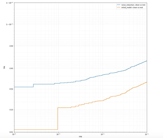 Figure 1. The partial receiver operating characteristic (ROC) for relabeled data (“noise reduction”) vs. noisy data (“initial model”) on the clean files
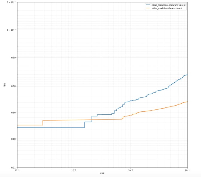 Figure 2. The partial receiver operating characteristic (ROC) for relabeled data (“noise reduction”) vs. noisy data (“initial model”) on the dirty files
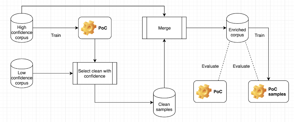 Figure 3. Training and evaluating the “POC” and “POC-samples” models
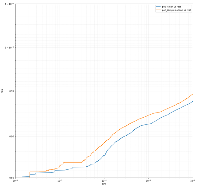 Figure 4. The “POC sample” trained on the clean samples-enriched dataset has much better performance than the previous “POC” model when evaluated by clean versus the rest
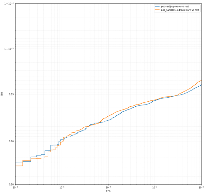 Figure 5. When it comes to adware/PUPware vs. the rest, both models have similar performance
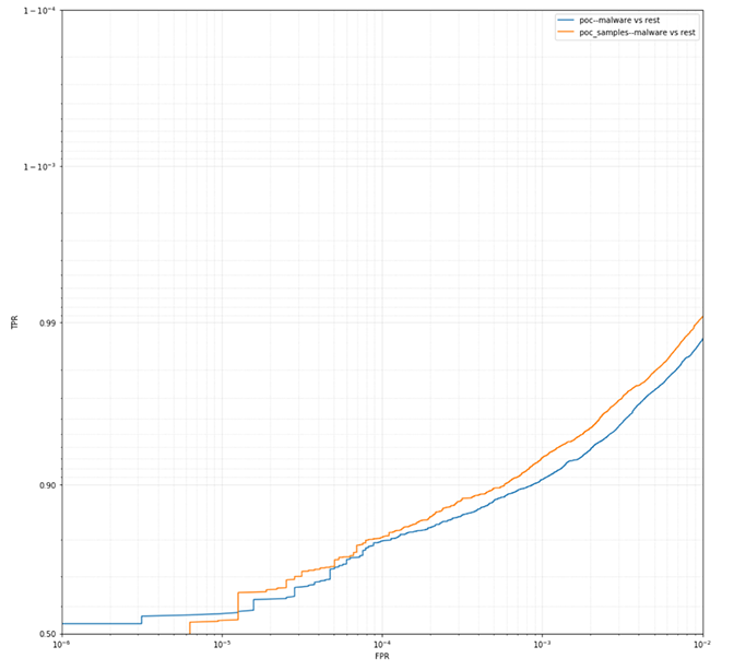 Figure 6. The results from malware vs. the rest also indicate the “POC samples” performed better than the “POC” model overall, with the exception of lower false positive rates. This is understandable because the models were only trained in 200 rounds for comparison purposes, using the parameters of a production model with no fine-tuning
By employing MOLD, we therefore speed up sample selection for training purposes (by reducing the volume that needs to be manually checked by experts) and help improve detection targets by enhancing the corpus with high-value samples from undersampled classes.
Figure 6. The results from malware vs. the rest also indicate the “POC samples” performed better than the “POC” model overall, with the exception of lower false positive rates. This is understandable because the models were only trained in 200 rounds for comparison purposes, using the parameters of a production model with no fine-tuning
By employing MOLD, we therefore speed up sample selection for training purposes (by reducing the volume that needs to be manually checked by experts) and help improve detection targets by enhancing the corpus with high-value samples from undersampled classes.
MOLD 101
First let’s begin by clarifying what we mean by label noise, where it originates, why it can lead to a detection performance hit to machine learning models, and how it can be detected and dealt with efficiently. Traditionally, machine learning algorithms and pattern recognition methods have been sorted into two broad groups: supervised and unsupervised (also known as “predictive” and “informative” in data mining terminology). The distinction boils down to whether training data (labeled samples) are available or not. Supervised classifier design is based on the information supplied by training samples. In this case, training samples consist of a set of training patterns and associations, instances or prototypes that are assumed to represent all relevant classes and bear correct class labels. Nevertheless, obtaining training data is not usually a trivial process. While for computer vision applications it can be relatively easy to manually label objects in an image, in cybersecurity space, however, class identification of prototypes is an extremely difficult, time-consuming and very costly task. This is because specialized knowledge or expertise is required to decide whether a computer file is adware or a truly malicious sample. As a consequence, some imperfectly or incorrectly labeled instances(aka label noise or mislabeling) may be present in the training corpus, leading to situations that fall between supervised and unsupervised methods. These situations are also known as imperfectly supervised environments.
Label Noise
Label noise is often categorized loosely into random and non-random noise. The distinction between the two is that random noise distribution does not depend on input features, whereas non-random noise is more general and is influenced by input features. While random label noise is easier to mathematically model, non-random label noise is far more prevalent in real-world scenarios, such as malware classification tasks. Label noise modeling can be further grouped into local and global approximations, based on model granularity. Local approximations are more flexible, as they treat label noise individually, i.e., for each data point or training instance. One way to achieve this in the case of logistic regression is by including a shift parameter in the sigmoid function. The shift parameter controls the cutting point of the posterior probabilities of the two classes. However, this sort of local approximation to model label noise becomes computationally expensive with increases in the number of training samples, and it is prone to overfitting issues. Instead, an alternative is a global approximation where the label flipping probabilities are summarized by one statistic (e.g., the flipping probability is the same for all instances in the same class). But such a global random noise label model is inevitably too restrictive — encountering underfitting issues. Generalization accuracy of the learning algorithm may be degraded by the presence of incorrectness or imperfections in the training data. Particularly sensitive to these deficiencies are nonparametric classifiers whose training is not based on any assumption about probability density functions. This explains the emphasis that machine learning and pattern recognition communities place on the evaluation of procedures used to collect and clean the training sample — critical aspects for the effective automation of discrimination tasks.Prevent MOLD From Growing
Some of the more complex Portable Executable (PE) file classifiers we’ve developed learn from tens of thousands of features. Given the high dimensionality of the data sets, a good starting point to evaluate label noise is experimenting with generic linear models, which are designed to be resilient to various degrees of noise level. One such example is the generalized logistic regression model proposed by Bootkrajang (see: “A Generalised Label Noise Model for Classification in the Presence of Annotation Errors” for details), where the likelihood of the label flipping is modeled by an exponential distribution using latent variables. The idea behind this model is that points closer to the decision boundary have relatively higher chances of being mislabeled than points farther away. The advantages of this particular label noise model are that it’s flexible enough to deal with both random and non-random label noise, and also simple enough to avoid the curse of dimensionality (the number of parameters is still based on number of classes rather than number of training samples). On the downside, one needs to make further assumptions to try to stabilize the convergence of the loss function. Therefore, training this generalized logistic regression requires implementing a specific chain of parameter updates and sometimes a bit of luck — some features in our data sets have unusual distributions that do not always work particularly well with this model. According to Bootkrajang, the generic logistic regression model works better than other similar robust linear models published in the literature, particularly when label noise levels (naturally occurring or artificially created) vary between 10% and 40%. With some of our data sets, though, a significant improvement in performance is not immediately apparent when using Bootkrajang’s model versusregularized “vanilla” logistic regression models. We believe the most likely explanation for this result is that our data sets have low levels of label noise — but the generic logistic regression model’s performance on very high dimensionality sets has not been reported previously. Our samples are carefully tagged using bespoke labeling utility pipelines, and the maximum level of noise estimated on new samples is therefore generally pretty low. The exact figures vary depending on the label noise modeling approach. For example, using linear models, the estimated level of noise does not usually exceed 2% for particularly tricky-to-classify data sets. Further MOLD experiments we carried out were based on ensemble models. Using unanimous voting, the ensemble models estimated an upper bound of 0.5% for the label noise level on one dataset (700,000 samples with a population of roughly 10% clean, 80% malware and 10% adware or PUPware). Balancing hyper-parameter tuning results with training time and model complexity for datasets of under 1 million samples, one of the best-performing ensemble models used instance-based models as estimators (in particular, the ensemble involved 20 base estimators, a random feature subsampling of 0.05 and a bagging fraction of 0.3 for sample selection). Instance models were trialed due to their ability to adapt to previously unseen data, and also their sensitivity to label noise in particular. Although using an ensemble solved the overfitting problem of single-instance-based learners, one big caveat still remained: the scalability issue, i.e., the growth of models along with the size of the training corpus. To address this, pruning techniques are normally used.
Condensation Issues
Condensing (pruning) algorithms is aimed at improving the performance of the resulting systems by discarding outliers and cleaning the overlap among classes. In doing so, these techniques are fundamentally looking to filter the training prototypes, but as a byproduct, they also decrease the training set size, and consequently reduce the computational burden of the classification method. Let’s take Hart’s algorithm, for example. In this case, a sample x from the training set T is removed from T and added to the prototype set U, if the nearest prototype in U has a different label than x. This process continues until no more prototypes can be added to U. Therefore, using the nearest neighbor rule (k=1), the prototype set U can be used instead of the entire training set T to classify a sample without a performance hit. A few other proposals aim to modify the structure of the training sample by correcting the label of prototypes assumed to be initially mislabeled using k-NN rules with multiple k values. Some condensing algorithms are more or less inconsistent, though. For example, among Hart’s algorithm caveats are that the results depend on the order in which the instances are assessed, the prototypes near the decision boundaries are not preserved, and all of the superfluous inner training cases are not eliminated. The shortcomings of Hart’s algorithm are addressed by other methods in the literature. A more consistent approach to evaluating a data point’s worth is by employing the Shapley value theory. The most common use case for the Shapley value is feature importance, which we previously described here. The Shapley value theory can also be used when evaluating label noise. The assumption here is that the adverse impact that mislabeled data have on training and evaluating models can be traced down to the lower Shapley values (e.g., sometimes negative values are included). See Ghorbani and Zou for more details. We have applied the Shapley value to a small subset of up to 100,000 samples in one of the static models for in-memory classification. Depending on the quality of the feature vectors used, results can vary. The following plots show the improved performance of a sample research model once the noisy labels have been relabeled (Figures 1 and 2). Figure 1. The partial receiver operating characteristic (ROC) for relabeled data (“noise reduction”) vs. noisy data (“initial model”) on the clean files Figure 2. The partial receiver operating characteristic (ROC) for relabeled data (“noise reduction”) vs. noisy data (“initial model”) on the dirty filesMOLD Remediation
The primary use case for MOLD is to automatically identify mislabeled data, and as a consequence, monitor label noise levels in our datasets. For research purposes, though, we keep MOLD lightweight compared to our most complex static malware detection models. Therefore, a secondary use case for MOLD is to contribute to pre-screening new, unseen samples before selecting them for corpus enhancements. Often, we use MOLD together with other specialized but similarly lightweight models. We do this using a stacked ensemble architecture to improve the confidence in our final decision. For validation and monitoring purposes, samples from all of our defined confidence bands are randomly selected for expert hash reviews — for example, from a batch of millions of hashes, thousands are subsampled. Samples detected with lower confidence are particularly important, as they can have a high Shapley value. Therefore, including them in the subsequent training iterations can often further improve the performance of our models at the tail ends. Below we present some of the results we had with MOLD in a proof-of-concept (POC) experiment. In this scenario, we had an abundance of mostly clean samples gathered by one of our proprietary systems developed by CrowdStrike cybersecurity threat engineers. The tagging of these particular samples was done automatically using simple heuristics, and we, therefore, had lower confidence in the individual labels — we’ll call this the “cleanish” data set. We wanted to make use of these additional samples to improve detection rates and reduce false positives in some of our static classifiers, especially with regard to the clean samples. To this end , we used a MOLD model (“POC” in Figure 3) trained on a completely different subset of data (around 6 million PE files) for which we had a higher confidence in terms of labeling. The POC model was then used to select clean samples from the larger “cleanish” dataset. We then trained another model (“POC samples”) on this enriched data set to compare performance. The additional clean samples were selected from the “cleanish” dataset at the 0.9 threshold (around 4 million clean samples selected, resulting in 10 million samples for the enriched corpus). Figure 3. Training and evaluating the “POC” and “POC-samples” models Figure 4. The “POC sample” trained on the clean samples-enriched dataset has much better performance than the previous “POC” model when evaluated by clean versus the rest
Figure 5. When it comes to adware/PUPware vs. the rest, both models have similar performance
Figure 6. The results from malware vs. the rest also indicate the “POC samples” performed better than the “POC” model overall, with the exception of lower false positive rates. This is understandable because the models were only trained in 200 rounds for comparison purposes, using the parameters of a production model with no fine-tuningKeeping It MOLD-proof
As we have shown, MOLD techniques allow us to further improve the accuracy of our models. These techniques can help by both reducing existing label noise and also allowing the addition of more labeled instances automatically. To tap into this potential, we are enhancing our training labeling utility pipelines by adding automatic MOLD detection techniques. Given the encouraging MOLD results on static detections so far, we plan to leverage these techniques we’ve developed to push the performance boundaries of the full range of our malware detection models. Are you an expert in designing large-scale distributed systems? The CrowdStrike Engineering Team wants to hear from you! Check out the openings on our career page.Additional Resources
- Learn more about the CrowdStrike Falcon®® platform by visiting the product webpage.
- Learn more about CrowdStrike endpoint detection and response by visiting the Falcon InsightTM webpage.
- Test CrowdStrike next-gen AV for yourself. Start your free trial of Falcon Prevent™ today.


