


![Helping Non-Security Stakeholders Understand ATT&CK in 10 Minutes or Less [VIDEO]](https://assets.crowdstrike.com/is/image/crowdstrikeinc/video-ATTCK2-1?wid=530&hei=349&fmt=png-alpha&qlt=95,0&resMode=sharp2&op_usm=3.0,0.3,2,0)
![Qatar’s Commercial Bank Chooses CrowdStrike Falcon®: A Partnership Based on Trust [VIDEO]](https://assets.crowdstrike.com/is/image/crowdstrikeinc/Edward-Gonam-Qatar-Blog2-1?wid=530&hei=349&fmt=png-alpha&qlt=95,0&resMode=sharp2&op_usm=3.0,0.3,2,0)


?wid=2048&hei=1350&fmt=png-alpha&qlt=95,0&resMode=sharp2&op_usm=3.0,0.3,2,0)


- CrowdStrike researchers use machine intelligence to categorize zero-day malware by using behavioral data, pre-defined Threat Type groups, and supervised and unsupervised clustering and similarity assessment.
- The conventional approach of assigning a family name and attribution to new and unknown (zero-day) malware for categorization is not sufficiently accurate and causes a delay in defending against newly discovered malware due to the reliance on manual human analysis.
- CrowdStrike’s new method automates the process of identifying the Threat Type of zero-day malware with a measurable degree of confidence, enabling a quicker response to mitigate threats.
Classifying new and unknown (zero-day) malware has always been a challenge in the security industry as new variants are discovered in the wild at an overwhelming rate. Underlying questions asked for each new and unknown malware instance include: “What is it?” “What threat does it represent?” and “How can we protect ourselves?”
Categorizing zero-day malware traditionally starts by assigning a malware family name and, when possible, attributing the malware to a threat actor. But understanding the true threat zero-day malware represents to organizations requires a deeper understanding of the actual malware capabilities when it’s first discovered.
CrowdStrike researchers automate the process of identifying Threat Types to enable rapid zero-day classification for unknown malware and solve the malware family name challenge.
Malware Family Name Bing
A common method of attempting to categorize new malware is to determine its family membership. Traditionally, that involves manual analysis by researchers, and sometimes, especially with zero-day malware, that preliminary analysis can lead to misattributing the unknown malware to the wrong family. For example, in 2017, in a rush to label a new and unknown destructive malware that later became popularly known as NotPetya, several researchers attributed the malware to the Petya and WannaCry ransomware families.
Zero-day malware attribution can also be expressed through a vendor-supplied malware family name such as those returned by VirusTotal. A look at the results for a malware sample may show a variety of names, which is not ideal.
For example, consider a sample with the following hash:
2627b94804ac67efd9e68c19fcd18577c908cb5230ea92c3c576ff4a840bcfd8
VirusTotal shows several names for this sample, but Microsoft’s naming convention (which uses the Computer Antivirus Research Organization’s malware naming scheme) identifies this as a variant of Fuery (Trojan:Win32/Fuery.C!cl), as shown in Figure 1.
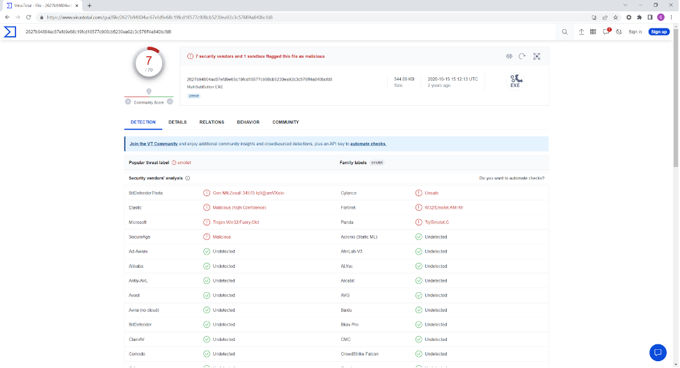 Figure 1. Screenshot of sample naming by Microsoft, as shown in VirusTotal (click to enlarge)
Interestingly, the sample with the below hash has identical behavior:
7728093295f3028320dc5c891364324fa5432c7af840fedf91cbc6757ee02881
However, most security vendors (including VirusTotal and Microsoft) consider this a variant of Emotet
(Trojan:Win32/Emotet.DEO!MTB), as shown in Figure 2.
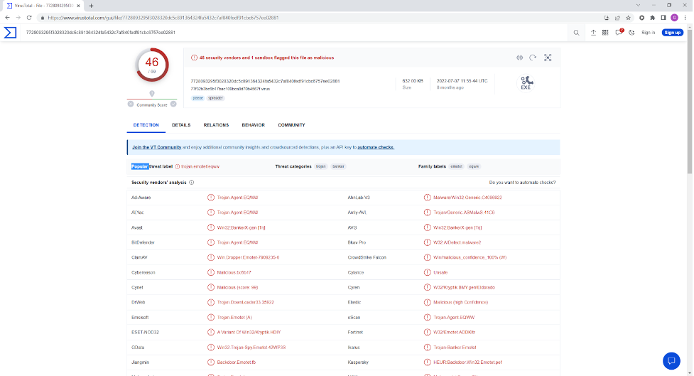 Figure 2. Screenshot of sample naming by Microsoft, as shown in VirusTotal (click to enlarge)
So which is it, Fuery or Emotet?
Vendors often use generic detections, which can result in name ambiguity and overlap. The previous example — where the hash was detected as an Emotet variant by some security vendors, while others didn't detect it at all — exemplifies this issue. Thus, agreeing on a family name for newly detected malware can be a challenge. Furthermore, an analysis of malware family names in VirusTotal revealed over 1,100 different names in use, even when normalizing them. This means there are instances where different malware samples exhibit identical or extremely similar behavior but are given completely different family names, making the naming of families irrelevant in some cases.
Figure 3 is an overview of the distribution among a subset of normalized (consensus) malware family names.
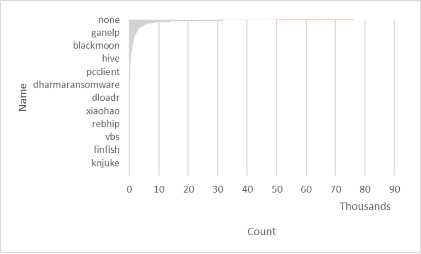 Figure 3. Pivot chart showing the distribution across a set of normalized VirusTotal malware family names (click to enlarge)
The chart is constructed to highlight changes in the slope of the count. The chart is heavily skewed by the “none” category, where a normalized consensus name couldn’t be generated.
Another issue with malware family names is that they depend on a consensus of third-party results, which is what VirusTotal reports. This means new and unknown samples will not have naming until that consensus is reached — a process that can take days at a minimum, and often weeks or even months.
Automated malware analysis is almost always limited to using static features. Few systems use runtime (or behavioral) data, as this is much harder to collect than retrieving static features, such as from a file or even a captured command line. Runtime analysis depends on the sample replicating, but often it won’t in analysis and detonation environments.
Automating Zero-Day Malware Classification
Our solution involves a series of components aimed at improving threat detection. To start, concise and easily understandable Threat Type groups are generated to aid in the identification of malware groupings. Next, new samples are compared to group centroids to assess their similarity.
To further enhance the determination of Threat Type groups, a multi-class classifier is used. And, unsupervised clustering will be utilized to generate sub-centroids within the Threat Type groups. The solution provides lists of nearest samples based on centroid comparisons. The primary dataset used is behavioral data, but it can be optionally used alongside static data for hybrid comparisons. The combination of these components aims to improve the accuracy of threat detection.
Having a reliable similarity assessment system that can operate on unknown samples means being able to answer our questions — “What is it?” “What threat does it represent?” and “How can we protect ourselves?” — with a measurable degree of confidence. And by establishing similarity with lists of other samples, prior in-depth analysis of these can be used to better understand the new sample — without it first needing to be examined in depth by human analysts (which can introduce delay).
Defining Threat Type Groups
To address the issue of malware sample classification, we developed a solution that involved organizing the samples into a set of small groups. We carefully selected an initial list of 15 groups that encompassed a wide range of threat types while remaining easy to understand. The groups included categories such as Adware, Application, Backdoor, Banker, Clicker, CoinMiner, Downloader, Dropper, Exploit, GameThief, HackTool, Keylogger, Password Stealer, Ransomware, and Trojan Spy. These groups provide a simple and intuitive way to categorize malware samples, making it easier to identify and respond to potential threats.
This was just the initial set, used for analysis. Later expansion added two more groups — Worm and Virus —for illustration, not included in the results.
The distribution of samples within the 15 groups is not uniform, as expected. The data below shows the similarity of the farthest group member (with a range of 0 to 1, with 0 being the lowest) for the initial set of Threat Type groups:
- Adware: 0.24
- Application: 0.26
- Backdoor: 0.15
- Banker: 0.37
- Clicker: 0.39
- CoinMiner: 0.26
- Downloader: 0.21
- Dropper: 0.17
- Exploit: 0.28
- GameThief: 0.40
- HackTool: 0.31
- Keylogger: 0.34
- Password Stealer: 0.21
- Ransomware: 0.00
- Trojan Spy: 0.28
Finding the Right Features Using Behavioral Data
The system utilizes behavioral data that can be obtained from sample detonations in a sandbox system and/or from field behavior collection, to create a feature vector (FV) from the collected features from a sample. To make the data more suitable for machine learning and similarity systems, we used one-hot encoding, which transforms each categorical value into a unique feature that can be set or not, creating a wide feature space (sparse dataset) with most features not set. Consequently, the data becomes sparse and high-dimensional, which is usable by similarity functions.
Example of sample FVs and their similarity (Cosine):
hash:                 77a860ac0b7deb3c17acba8d513a5574069070153274925e6f579d22724544fc


feature vector:   1427,1428,4795,5012,6088,7049,11091,11092,11093,12160,12170,12200,12207,12249,12252,14401,14410,14411,14412


hash:                 08d12841527cd1bb021d6a60f9898d6e0414d95e7dcde262ed276d5c8afa33cc


feature vector:   1427,1428,4795,5012,6088,7049,11091,11092,11093,12155,12160,12170,12200,12205,12207,12249,12252,14354,14401,14410,14411,14412

Similarity: 0.93
These samples have nearly identical features, resulting in a high similarity assessment.
Using Similarity Comparison to Achieve Shortest Single Match Wins
For our purposes, we simplified the similarity or distance comparison functions and limited them to cosine distance, which measures the angle between feature vectors. It is a robust method of measuring similarity and has an added benefit of inherent normalization of results within a range (1 indicating identical features, 0 indicating no similarity).
To compare similarities, we created centroids for each group of Threat Types by selecting group members with the lowest average distance to all other members. When a sample is submitted, we generated its feature vector and compared it to the feature vectors of the centroids to determine its similarity distance. We used the "shortest single match wins" approach where the comparison with the smallest distance is chosen as the closest, meaning we selected the nearest centroid. This allowed us to identify the likely Threat Type group the sample belongs to and determine the confidence of our assessment based on the similarity distance.
We noted (in a datastore/database) the Threat Type group the submitted sample was determined to be a member of and its distance from that group’s centroid.
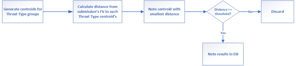 Figure 4. Chart with the overall processing flow for determining the Threat Type group for an analyzed sample (click to enlarge)
Generating a List of Nearest Samples
To find the most similar group of threats to a newly submitted sample, we started by determining the closest match based on previously identified Threat Types. This match served as a starting point for our search, and we then looked at other members of this Threat Type and how similar they are to the submitted sample. We repeated this process with other Threat Types until we had a list of the closest matches to the submitted sample. By doing this, we can quickly identify potential threats and take action to protect against them.
Unsupervised Clustering
The above centroid-based approach is an application of supervised training and clustering, where we had a set of training and testing samples already labeled as members of a Threat
Type group. It proved valuable to also include unsupervised clustering. We also used K-means clustering using the “elbow method.” K-means is a simple yet robust system for clustering, with the limitation that it requires choosing the number of clusters separately. The elbow method plots distortion of the clustering results vs. the number of clusters. In an optimal situation, the plot highlights the “elbow” where the distortion flattens out, indicating the optimal choice for the number of clusters.
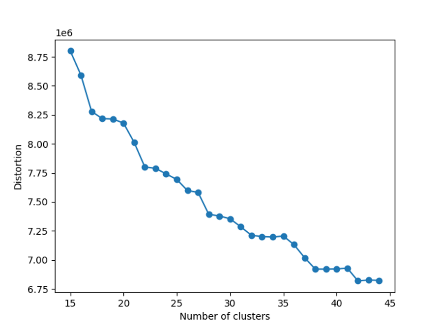 Figure 5. Chart with the distortion plot for the unsupervised K-means clustering application to our feature set (click to enlarge)
The graph in Figure 5 shows there is no clear point where the curve bends, but it does start to level off. It would be too time-consuming to plot the curve for more than 400 clusters, so we stopped there and found that the curve continued to level off. Based on this, we chose to use 400 clusters.
Supplementing with a Multi-Class Classifier
We applied a multi-class classifier to the 15 Threat Type groups, which proved very accurate when combined with a limited set of static features.
The multi-class classifier serves as a means of confirming the Threat Type group membership of a sample and its agreement with the similarity matching enhances the confidence of membership in the determined group. However, if there is no agreement, the similarity-based determination may still be used, but without an added confidence boost reported.
Although useful, this method could not be effectively applied to the 400 sub-clusters generated via K-means because the per-cluster data becomes too sparse at those cluster counts, making it limited to the small set of Threat Types group clusters (15 at the time).
The Importance of Understanding the Shape of a Cluster
Understanding the shape of the clusters is valuable because it helps us find answers to questions such as: Are members of the cluster tightly packed around the centroid? Are they distributed evenly and thinly? Do they form clumps or sub-clusters within the larger cluster? How adjacent and overlapping are the clusters to each other?
To better understand the shape of the clusters, we looked at several things. These include how far each member of a cluster is from the center of that cluster, how far the member that is farthest from the center is, how far each cluster's center is from the centers of other clusters, how far members of one cluster are from the center of another cluster, and the best number of clusters to use. By examining these aspects, we gain a better understanding of the clusters and how they are related to each other.
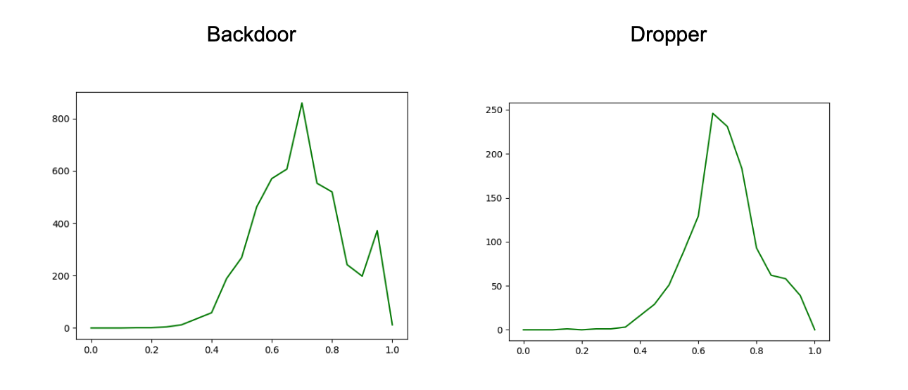 Figure 6. Charts with the distribution of distances between cluster members and the cluster centroid, for subset of the Threat Type groups (click to enlarge)
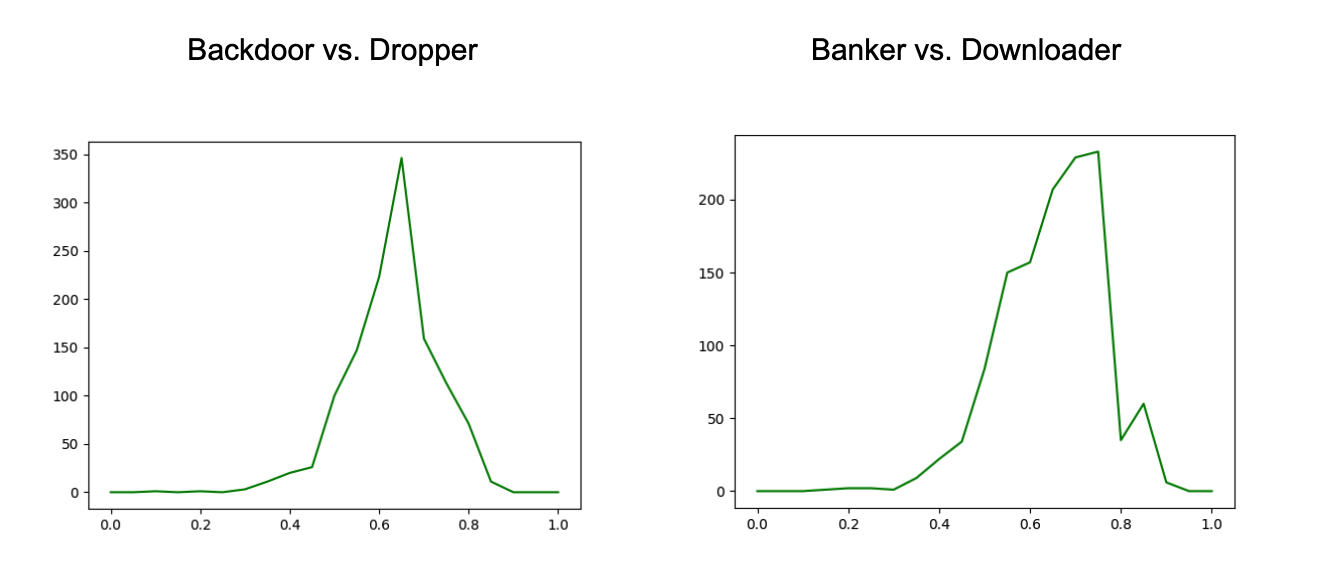 Figure 7. Charts with the distance distributions comparing members of one cluster and centroid to another (click to enlarge)
These distribution charts show that the samples within a Threat Type group don’t all cluster around the group centroid, and even between a group’s members and another group’s centroid, there is a decent amount of similarity. All of this reinforces the value of generating sub-clustering with an unsupervised method, as noted earlier, and then using these sub-clusters in assessing similarity.
Measuring Efficacy
Similarity System
First, we used the centroids from the 15 threat type groups and found that the system worked well when the similarity between samples reached .92 or greater. Then, we added a more detailed analysis by looking at the centroids from the 400 sub-clusters generated using unsupervised clustering. This method has a higher false positive rate at lower similarity, but higher starting true positive and determination rates. We found that using both methods together — including the unsupervised centroids’ results after the .92 similarity threshold and only using the unsupervised set before that — produced the best overall result. Figure 8 shows how this hybrid method performed.
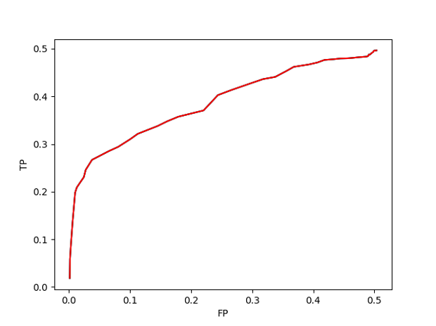 Figure 8. Chart showing the hybrid ROC (Receiver Operating Characteristic) curve (click to enlarge)
We evaluated the similarity system's efficacy by comparing its Threat Type group membership determination to the actual membership for a set of samples. At lower similarity thresholds, there was increased adjacency and overlap between members of different groups, leading to decreased accuracy, as shown by the ROC curve. However, since the system's goal is to assess similarity rather than classify, this level of accuracy is acceptable, as the system generates lists of similar samples with confidence scoring. Figure 9 shows the determination rate against the similarity threshold, with only centroids as the comparison set.
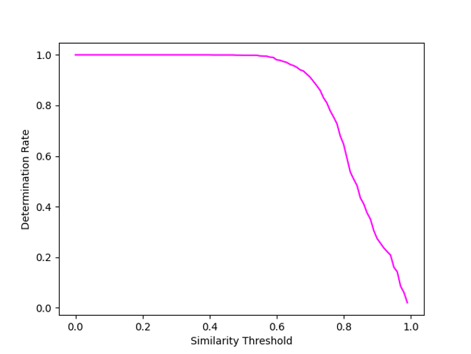 Figure 9. Chart with the determination rate against the similarity threshold (click to enlarge)
Past a similarity threshold of ~0.6, the system quickly stops finding similar samples, which is not unexpected. In the random sets of samples used for testing and the generated centroids, there would generally be a centroid in the comparison set closer than 0.6 similarity.
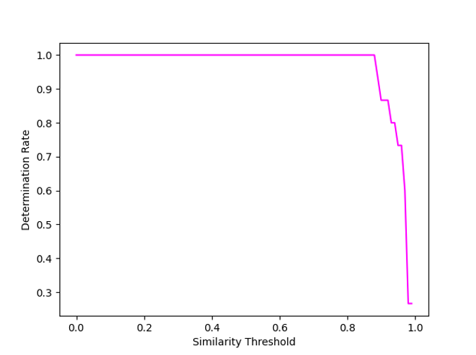 Figure 10. Determination rate chart with the sub-centroids used for the comparison set (click to enlarge)
The second chart illustrates why having the sub-centroids in the comparison set facilitates extended similarity accuracy at lower thresholds and why including these sub-centroids facilitates locating the closest samples to the submitted sample.
Multi-Class Classifier
The multi-class classifier (against the Threat Type group clusters) — built with XG Boost and using behavioral data alone — produced good results, as shown below.
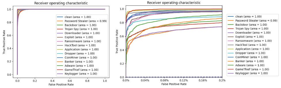 Figure 11. ROC charts with the multi-class classifier performance results (click to enlarge)
That classifier produced much better results when the behavioral data was combined with a subset of static feature data.
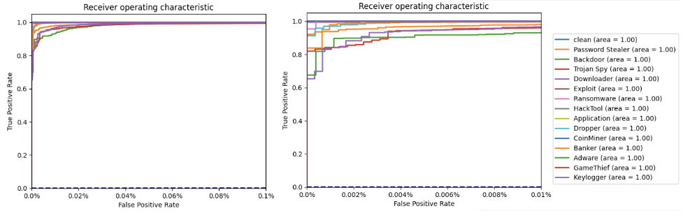 Figure 12. Charts with the classifier performance combining behavioral data with a subset of static feature data (click to enlarge)
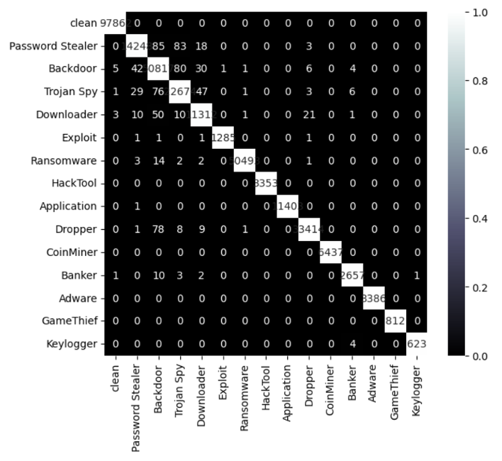 Figure 13. Confusion matrix for the multi-class machine learning using the hybrid behavioral and static data (click to enlarge)
The confusion matrix (Figure 13) helps us evaluate the performance of the classification algorithm. It shows a comparison between actual and predicted values with 15 classes. Predicted labels are on the X-axis, and the true labels of our test set’s samples (the prediction was done using only the test set) are on the Y-axis. Ideally, a perfect classifier would only have values on the diagonal, which would mean all of the test samples were correctly classified for all 15 classes. The confusion matrix shows that multi-class models based on behavioral and static data could be extremely accurate and provide valuable insights into what the Threat Type is for an unknown sample.
T-SNE Visualization
T-SNE (t-Distributed Stochastic Neighbor Embedding) is a technique for visualizing high-dimensional data in a low-dimensional space. It can help to reveal patterns and relationships that may not be immediately apparent from looking at raw data. T-SNE works by mapping the high-dimensional data points to a lower-dimensional space in a way that preserves the local relationships between the points. It does this by maximizing the likelihood that similar data points will be mapped close to each other in the lower-dimensional space, while dissimilar data points will be mapped farther apart.
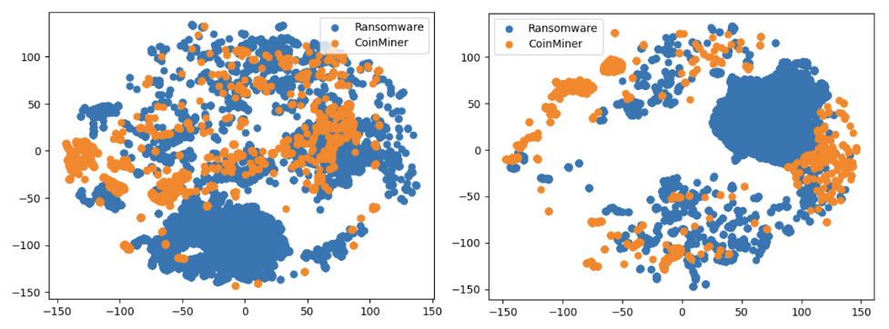 Figure 14. T-SNE visualization of Ransomware and CoinMiner Threat Type groups (click to enlarge)
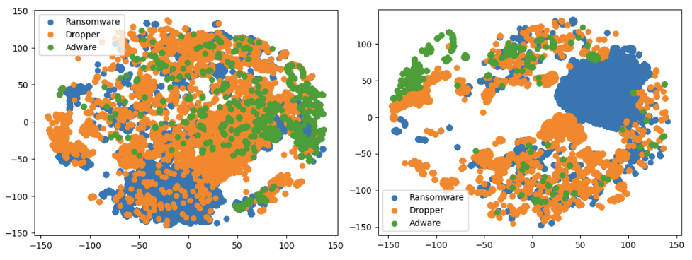 Figure 15. T-SNE visualization of Ransomware, Dropper and Adware Threat Type groups (click to enlarge)
We used T-SNE to visualize the data into a lower-dimensional space and demonstrate the model's ability to separate Threat Type groups. Although T-SNE does not preserve distances or density, it helps visualize data and identify patterns. T-SNE also shows when classes are mixed and not easily separable, as seen in the second example where Adware and Dropper show some intertwining. However, these examples also illustrate the challenges in visualizing this type of data.
Strengthening Customer Protection with Effective Zero-Day Malware Threat Mitigation
Understanding the type of cybersecurity threat is crucial as it helps in taking appropriate measures to protect customers from zero-day malware. Each type of threat requires a unique approach to defense and protection, and knowing the threat type helps to prevent and mitigate the threat while prioritizing security efforts.
A similarity system that combines pre-defined Threat Type groups and unsupervised clustering-generated sub-centroids is effective at identifying malware, zero-day malware and threat groups, including for unknown samples. Combining this with a multi-class classifier provides added confidence in Threat Type group identification, allowing for faster and more effective responses to new malware threats, without requiring human analysis or community consensus, to more effectively and efficiently stop breaches.
Additional Resources
- Learn more about the CrowdStrike Falcon platform by visiting the product webpage.
- Learn more about CrowdStrike endpoint detection and response by visiting the CrowdStrike Falcon Insight XDR webpage.
- Test CrowdStrike next-gen AV for yourself. Start your free trial of Falcon Prevent today.