CrowdStrike Researchers Explore Contrastive Learning to Enhance Detection Against Emerging Malware Threats

January 22, 2025

| | AI & Machine Learning
  • CrowdStrike research shows that contrastive learning improves supervised machine learning results for PE (Portable Executable) malware
  • Applying self-supervised learning to PE files enhances the effectiveness of machine learning in cybersecurity, which is crucial to address the evolving threat landscape
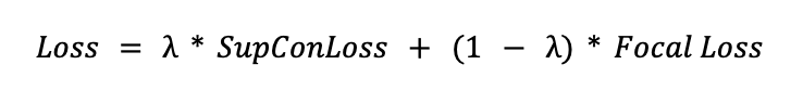
  • CrowdStrike researchers engineered a novel loss function to optimize contrastive learning performance on imbalanced datasets

The process of crafting new malware detection features is usually time-consuming and requires extensive domain knowledge outside the expertise of many machine learning practitioners. These factors make it especially difficult to keep up with a constantly evolving threat landscape. To mitigate these challenges, the CrowdStrike Data Science team explored the use of deep learning to automatically generate features for novel malware families.

Expanding on previous CrowdStrike efforts involving the use of a triplet loss to create separable embeddings, this blog explores how you can use contrastive learning techniques to improve upon this separable embedding space. 

Furthermore, we will discuss a novel hybrid loss function that is capable of generating separable embeddings — even when the data is highly imbalanced.

What Is Contrastive Learning?

Contrastive learning techniques have had many successes as a self-supervised learning algorithm in the natural language processing and computer vision domains. 

The goal of these techniques is to contrast different samples, such that similar ones are closer together and dissimilar ones are farther apart from one another — similar to how we as humans differentiate objects by comparing and contrasting them.

Over time, as we develop, we can differentiate things based on features we identify. For example, we can tell the difference between a bird and a cat based on features such as a bird having wings and a cat having pointy ears and a tail.

We can train a deep learning model to automatically capture these features by applying a contrastive loss function. This is generally done using a Siamese network, where two identical networks are fed different data. The networks are then trained with a loss function used to measure the similarity between the two inputs.

Below, we detail examples of contrastive learning techniques. 

SimCLR

The Simple Contrastive Learning (SimCLR) framework is an algorithm developed by researchers at Google Research (formerly Google Brain). It works by applying augmented versions of the same image through a deep neural network, where the goal is to maximize agreement between these images. The framework is depicted in the image below (Figure 1).

Figure 1. SimCLR representation (from “A Simple Framework for Contrastive Learning of Visual Representations,” Google Research) Figure 1. SimCLR representation (from “A Simple Framework for Contrastive Learning of Visual Representations,” Google Research)
This technique has three main components: image augmentation, a deep neural network and a contrastive loss function. It works by taking an image and applying a random augmentation to it (such as cropping, rotating, flipping, grayscaling, etc.). Afterward, the original image and its augmented version are inserted into the deep neural network to generate two vector representations. The loss function (Figure 2) is applied to a batch of images and their augmented versions. The function's goal is to maximize the cosine similarity between the pair and minimize cosine similarity between all other samples in the batch.
Figure 2. Contrastive loss function (from “A Simple Framework for Contrastive Learning of Visual Representations,” Google Research) Figure 2. Contrastive loss function (from “A Simple Framework for Contrastive Learning of Visual Representations,” Google Research)

Supervised Contrastive Learning

One problem that arises with the SimCLR framework is the need to use large data batches in order for it to produce the desired results. As a result of using a large batch, there may be multiple samples of the same class label. If this happens, the algorithm will try to push these samples away from one another. 

If label information is available, then using the supervised version of this algorithm may be the better choice. Supervised contrastive learning (SupCon) is an algorithm that incorporates label information into the loss function. This algorithm works by maximizing cosine similarity between samples in a batch with the same label, rather than just pairs. In addition, it minimizes the cosine similarity between samples of different labels.

Discussed in our previous research, a triplet loss was used to develop the vector space with separable malware families. Triplet loss thrives on choosing a pair of positive and negative samples, which the model has difficulty separating. SupCon builds and improves upon this technique by incorporating large batches during model training. Instead of relying on a single negative and a single positive sample, we now randomly sample a large number. By contrasting a large number of positive and negative samples, this method alleviates the issue of having to perform hard negative sample mining.

Contrastive Learning for Imbalanced Data

Focal Loss

As discussed earlier, we can generate an embedding space for different malware families even when the data is highly imbalanced. The class imbalance problem has plagued machine learning models, and data techniques like over/under sampling are used to try and remedy this issue. Instead of adding synthetic data or removing samples from our data set, we can apply a loss function to get the model to “focus” on samples that are hard to learn. Doing so allows us to utilize all of our data.

Focal Loss was developed by Facebook Artificial Intelligence Research (FAIR) for object detection. One problem that has been noted in object detection is that labels are very sparse and as a result, objects often appear in certain regions of the image but do not exist in the majority of the image. Focal Loss is an augmented version of cross entropy (CE) loss where the gradient of the loss function changes with respect to how hard it is to detect a sample. When we have a class imbalance, the model is able to easily identify the majority class while misclassifying minority classes. When we increase the gradients for the harder samples, the model will focus on classifying them correctly.

Figure 3. Focal Loss Function (original image from “Focal Loss for Dense Object Detection,” Facebook AI Research) Figure 3. Focal Loss Function (original image from “Focal Loss for Dense Object Detection,” Facebook AI Research)

Hybrid Loss

To be able to generate a vector space while also focusing on samples that are more difficult to classify, we developed a novel hybrid loss function. The function works by calculating the loss for both the SupCon and Focal Loss functions. The two losses are then weighted using a user-defined parameter 𝜆.

Convolutional Neural Networks Ingest Entire PE Files

Cybersecurity researchers have had considerable success in applying convolutional neural networks to raw binary files for classification. We take this approach by using an architecture inspired by the MalConv2 convolutional model. The temporal max pooling function creates the ability to feed an extremely long sequence to a neural network while keeping the memory footprint constant. 

Being able to feed in an entire binary without the problem of resources provides enormous benefit. This is an improvement over the methods used in our earlier work, in which the model ingests only 32KB of raw bytes starting from the entry point — a restriction imposed mainly to keep the memory and resources at minimum. Limiting the model to only learning from the entry point may discard important information pertaining to different PE file sections such as the header or import table.

The MalConv2 architecture consists of three main components: the embedding layer, the convolutional layer and the projection layers. We create a variation of the model architecture by applying a depthwise-separable convolution instead of the standard convolutional filter. This adaptation works in two steps. First, a depthwise filter is applied to each individual input channel. Next, a pointwise filter is applied to generate a linear combination of the depthwise filter output. This function reduces the number of parameters by 12x while maintaining the same performance. We believe this is due to the large convolution kernel sizes of 512 that we use. A kernel this large is likely able to learn many different features per individual filter. 

In order to use our hybrid loss function, we must retrieve multiple outputs from different regions of the network architecture, described in Figure 4. Once the entire input has been convolved and we have produced our temporal max pooling output, the dimension is compressed in half after each fully connected layer. The embeddings used for the SupCon loss are taken from our final fully connected layer, and the focal loss is taken from the final softmax output layer. The activation function used for all fully connected layers is the swish activation function.

Figure 4. Model Architecture Figure 4. Model Architecture

Contrastive Learning Applied to PE Malware

For the purposes of this research, our model was trained on a data set of roughly 15.5 million samples containing 500 different malware families. The number of samples from each malware family varied greatly, from 2 million samples for our most abundant family down to 655 samples. Figure 6 shows the embeddings produced by our network by reducing the fully connected dimension down to two using t-SNE (t-distributed stochastic neighbor embedding). 

For the purposes of visualization we chose a selected subset of ten different malware families to view from our testing data. These families were chosen based on how many samples there are in the training set. The common five families are: Ganelp, Padodor, CoinMiner, Dridex and Nabucur, each containing over 300,000 samples. The less common five — Emotetcrypt, Viking, xed-10, InstallMonster and Chinky — contain around 10,000 samples each. We attribute the ability to maintain sufficient separation between families of smaller sets by applying the focal loss to the network weights.

Figure 5. Embedding of malware families Figure 5. Embedding of malware families
Being able to manipulate the embedding space by providing labels can be extremely valuable. We decided to add an additional set of labels to see if we could move samples closer together based on more than one factor. Malware families have an additional higher-level class associated with their threat type. For example, worm, trojan, mineware and ransomware are various types of malware that have multiple families within each. We trained a model to not only separate PE files based on their malware family but also based on their threat type. This was achieved by applying the SupCon loss twice to the malware family and again to the threat type. The loss was then averaged between the two. Figure 6 shows 800 samples from 173 different malware families labeled by their threat type. We can see that it is not perfect but the majority of the samples fall in line with their threat type by training with the altered loss.
Figure 6. Embedding of threat types Figure 6. Embedding of threat types

Having the flexibility to move data around to various locations based on different criteria can be extremely powerful. Through this embedding space, it acts as a similarity space, where different files are clustered together by a given similarity criteria. When new files arise, we can get an idea on what type of threat they are by embedding the file, finding its nearest neighbors and extrapolating information from there. Given a sample that we have little information on, we can easily see if it has similarities to particular malware families as well as their overarching threat type. Future methods could involve shifting these embeddings around by their file type (exe, dll) or by which compiler was used.

Future Applications of Contrastive Learning

The main focus of this post was on training a model using the supervised approach. Labeling PE files can be a very expensive and time-consuming endeavor. Contrastive learning approaches appear to be a great candidate for self-supervised learning on PE files. Applying augmentations and gleaning information from the vast majority of unlabeled samples out there can be an extremely powerful tool if combined with fine-tuning for various downstream tasks. 

The cybersecurity threat landscape is continually evolving at a rapid pace, and machine learning is a crucial element in the defense against adversaries. The novel hybrid loss function developed by CrowdStrike data scientists will optimize contrastive learning effectiveness, a key method for improving supervised machine learning results against PE malware. Cutting-edge research such as this is a key element of the innovation that ensures the AI-native CrowdStrike Falcon® platform is always at the forefront of cybersecurity protection. Publishing the results is in support of CrowdStrike’s commitment to industry thought leadership, improving cybersecurity defenses globally against the threat of adversarial attack.

Additional Resources

Breaches Stop Here